Film curve plotting and fitting

[Mahler_one]

I too have been interested about the mathematics involved in determining some values on the film curve.

For me, the BTZS method of testing has placed the "density" of the negative correctly on the film curve most of the time. No person is always correct, and despite my best efforts, sometimes the negative appears too dense or too thin. I then try to correct my errors using the "correct" filters and/or paper grade(s).

In addition, while trying to learn how to develop film by inspection, I echo Nick's conclusion and those of so many others: Expose for the shadows, and develop for the highlights. Indeed.

 

[Lee L]

So it's a way to quantify results?

To do this within tolerable measurements you would have to use sheet film, so that each negative can be exactly calculated. With roll film I would think there are so much variation between frames that it's impossible to calculate a scientifically perfect way of processing the film, because the other 35 frames on your roll would be different in contrast, lighting, and exposure.

There are ways of getting around these issues. I have lately taken to photographing a 4x5 Stouffer 31 step wedge at not too high a magnification on a single frame of 35mm or 120 roll film. I include a lens extension factor if needed, but that's almost never necessary. I do not shoot full frame to avoid falloff and flare problems, backlight through milk glass and mask the Stouffer wedge carefully, and use full spectrum daylight balanced illumination.

To read the wedge densities, I project the negative on the enlarger baseboard and read densities with Darkroom Automation's enlarging meter. (Thanks for an excellent piece of hardware Nicholas.) This gives me excellent results and includes camera and enlarger effects.

The upside of this is that I can shoot a test negative on a single frame of a roll as a process control strip, saving time and materials. I have plans to make a light box specifically for using in this way, just putting the Stouffer wedge in a standard negative carrier and turning on the backlight would be the only setup work.

If I want to just make a couple of test frames for monitoring densities when I'm in the field, I use an ExpoDisc that I've had long enough that I can't remember what year I got it. That's usually a frame each for fb+f, a shadow zone, and a highlight zone of my choosing. Before the ExpoDisc came out, I used a milk-plex pre-exposure frame that I made from Ansel Adams' design.

Lee

 

[Thomas Bertilsson]

Lee, I understand how this would help you calibrate for normal lighting. If you shoot a roll of scenes in very high contrast you'd have to overexpose and compensate by contracting in processing to get optimal contrast for printing. How does the step wedge help here?

Or the next time lighting might be really flat, and you will find yourself underexposing and over-developing to yield normal contrast in your negative. The step wedge is going to look very strange indeed.

Either way. I'm definitely leading the topic of conversation astray. I was just curious to how the scientific helps in practical terms.

- Thomas

 

[Kirk Keyes]

I'm sorry if I'm sticking my nose where it doesn't belong, but does all this exercise really make your pictures better? Or is it an exercise in scientific curiosity? Or perhaps both?
If I took my photography to such scientific heights I think my head would explode. So I'm curious what drives the urge to go there.

Thomas - I think there is a point of diminishing returns on gaining more detailed knowledge in most any endeavour. Once you have the basics, you are often a long way there to mastering a subject - you know say 90 percent of the subject. Learning the next 9 percent takes more work, and the return on learing it is not as great as learning the first 90 percent. Learning the next 0.9% takes even more time and effort, and gives you little in return. Again, then next 0.09% takes yet more time and effort.

And on and on...

That said, some people, myself included, relish those little bits of information and the returns they often give. We enjoy the effort, we don't mind the time, and what we learn, is well earned.

Does it make us greater or better photographers, perhaps, but it also fulfills a need and desire to learn more about a subject we hold dear.

 

[Kirk Keyes]

Oh, and yes, some peoples heads do explode when certain subjects are invoked. For them, the old naysayer adage to just go out and shoot photos perhaps may actually be good advice for them. Afterall, taking photos is a lot more fun than having your head explode! (So I hear...)

 

[Kirk Keyes]

It looks pretty decent to me, and doesn't behave wildly outside the range of interest.

One thing I do when fitting curves to film data is to simply add more data points on the F+B end of the curve. Afterall, giving less exposure is not going to cause a decrease in F+B. So I just add extra points, all with the same density of F+B.

On the other end, since the films I use (Fuji Acros) is pretty linear and doesn't get a shoulder in normal usage/exposure, I add extra point to extend the data. I could just make a second step wedge exposure that is given several more stops and get real data, but I find the range of data I'm interested is well within the range of values I get for nearly all step wedge results I have. Only on really low contrast N-2 or less negs do I not get enough density to plot the data and make calulations from it. (That's because the neg density is not greater than the paper exposure range I use for grade 2.)

 

[Thomas Bertilsson]

Kirk, I really do understand about the desire to learn.

I think we like to learn about different aspects of the craft, and to a point I'd like to think that any knowledge we acquire about the craft will make us better prepared as photographers, perhaps even better as you state. Let's hope so.

For me there is no substitute for just 'doing', though. To develop empirical evidence of what works and what doesn't, to eventually be incorporated into a system of intuition where we don't even have to make calculations, but we learn to 'see' knowing what the outcome is going to be. That, to me, is real power and control. I am such a person that numbers don't do that for me, just repeated practice. To each their own. I respect your approach and I'm glad we're all a bit different.

- Thomas

 

[Kirk Keyes]

Well, all these schemes for various methods of testing are just different ways to get empirical evidence. And hopefully more accurate empirical evidence. Whether it's warrented, is up to the end user.

 

[RalphLambrecht]

... So here's another graph using Ralph's MGIV grade 2 data plotted in red, and a quick manual attempt to match it only at the highlights with a gaussian curve (in blue). It looks pretty decent to me, and doesn't behave wildly outside the range of interest. It also follows the procedure in Nicholas' post, and only tries to match one end of the curve. I haven't attempted to match the darker print densities...

Lee

I have tried to fit a normal distribution curve to paper data. It works reasonably well but falls short in the shoulder due to the bell curve's extreme peak.

 

[Stephen Benskin]

That said, some people, myself included, relish those little bits of information and the returns they often give. We enjoy the effort, we don't mind the time, and what we learn, is well earned.

I agree with Kirk. We should always encourage and support those who seek knowledge.

I can personally attest to the fact that my research has never kept me from shooting. Lack of money has kept me from shooting. I do sometimes wonder, however, if I should have had a better balance of my limited time with pursuing my art career or working on the direction of my art.

 

[Photo Engineer]

Evolution of this stuff

In post #247, Lee shows us an H&D curve with a bell shaped curve superimposed. If you consider the bell shaped curve to be representing the size frequency curve of the emulsion, then you see the reason behind a typical H&D curve.

This curve was idealized by H&D in the early days of photography (see my first figure below from Mees, Revised Edition). The best portion of the curve is marked in the figure.

In those days, that type of curve was not easily achieved due to the broad size frequency curves of emulsions made up to about the 50s. These were single run emulsions that produced the family of curves in my second figure below also from Mees. As addition times went up, speed went up but contrast went down. This was due to a broader distribution of grain sizes. Note how bowed the faster curves are. This made measurement and printing on faster films difficult at times.

In the 60s, it became possible to make double run emulsions that gave better speed, sharper toe and through blending, approached the H&D ideal.

In Haist, Grant shows how to utilize the ideal curve to optimize the Density Range vs the Exposure Range by the simple expedient of insuring that the exposure was off the toe or by giving it a slight overexposure of about 1/3 stop. See the 3rd and 4th figures below.

Unfortunately, in his text, Grant says that you should expose on the toe to compensate for flare, but I believe this was a typographical error, since flare reduces contrast and the toe is low in contrast, the combination would be very bad. I intend to discuss this with Grant in a few weeks while he is visiting Rochester and I'll report back on this.

Fortunately, in Mees, in the chapter written by J. L. Tupper, he ran tests in which a relatively straight line (or near ideal) film was used in-camera and in which flare was considered. This data, in the 5th figure, shows the areas of Just Acceptable prints and First Excellent prints. Even though there is overlap, the only portion of the curve (points Z - O) which are Excellent lie vitually completely on the derivative curve shown by Nicholas Linden in his earlier post.

In the final analysis, color films are built with a gamma of about 0.6 - 0.7 and most B&W films are built to that same range or up to .8 so that this flare factor can be compensated for, and they have long straight lines for long latitude, and interestingly enough, the individual color curves of many films reach a gamma of up to 0.8 through interimage effects.

Well, so much for a bit of history of the evolution of this topic.

PE

 

[Stephen Benskin]

I've just scanned the portion of the chapter Ron is referring to and will email it to anyone interested.

 

[dpgoldenberg]

So here's another graph using Ralph's MGIV grade 2 data plotted in red, and a quick manual attempt to match it only at the highlights with a gaussian curve (in blue). It looks pretty decent to me, and doesn't behave wildly outside the range of interest. It also follows the procedure in Nicholas' post, and only tries to match one end of the curve. I haven't attempted to match the darker print densities.

I don't think that this is actually what Nicholas was suggesting. As I understand it, he was arguing that the Gaussian functions should describe the derivative of the film curve, not the curve itself. The curve is then the integral of the Gaussian (for the appropriate region). This integral is known as the "error function", or "erf", because of its use in statistics. Unfortunately, erf does not have a simple closed form, and so fitting data to it requires first calculating numerical values.

Just to see what would happen, I tried fitting my function (see the first post in this thread) to just the first half of the error function. The results are attached. As you can see the fit is very good, certainly as good as any approximations used to justify the error function as a physically-based model. In addition, my function accounts for both the toe and an extended linear region with out patching together two functions. Accommodating the shoulder would require another function.

I also tried fitting my function to the toe and straight line region of Ralph's paper curve. The graph is attached, and, again, it works very well for this region.

I don't think that he meant it this way, but I think that Nicholas' post offers support for my approach, *for flim curves*.

David

 

[Lee L]

I don't think that this is actually what Nicholas was suggesting. As I understand it, he was arguing that the Gaussian functions should describe the derivative of the film curve, not the curve itself.

David

Yes, that is correct, and I took the same meaning, but perhaps got carried away with the gaussian vs polynomial issue. I need to review your code again after doing more reading, as I've been out and involved with other things most of the day. I'll see about correcting my earlier claims if I can still edit. (It's now too late to correct the post you're referring to here.)

My last math class was in 1973, and I'm not a mathematician or scientist, so I have to re-learn as I go when doing this kind of thing.

But my main point is that a curve derived from two gaussian functions for different shadow/highlight behaviors is more 'natural' (in the sense of scientifically 'elegant') than using a small section of a second order polynomial divided by a third order polynomial. The same objections that Nicholas has stated.

Lee

 

[RalphLambrecht]

In post #258, I showed that a bell curve works well for the paper toe and midsection but not the shoulder. Attached is an attempt to make it fit a film curve, which also does not work very well. Tmax does not have much of a shoulder over a 10-stop range, and the bell curve is trying to squeeze one in. How well it works may depend on the individual data, but I think, I'm better off with the nonlinear function I'm already using.

 

[Lee L]

Ralph,

Two points.

First, it's the integral of two bell curves (one for the toe, a different one for the shoulder, different behaviors near dmax and dmin) and a straight line that Nicholas has posted and PE has confirmed as the modeling standard established by researchers. That's not nearly the same as using a single gaussian distribution curve for the entire data set, which is what you're attempting in post #264.

Second, your film data in post #264 doesn't hit the shoulder, so you have no data above the straight line portion to fit to a shoulder curve model. Many modern films can go much further along the straight line portion than a 10 stop step wedge (properly exposed for the shadows) can accomodate with a single exposure. So you're trying to fit a single gaussian curve to toe and straight line data with no shoulder.

My guess is that dpgoldenberg's method would nail your TMX and TMY data. It does so for the similar data from my tests that I've tried it on. Try plugging his equation into Deltagraph and running a fit.

Attached is a 'two Gaussian' description of your paper curve just to show what happens to the toe curve at the shoulder and vice versa. As dpgoldenberg has noted, this is not the integral of two Gaussian curves plus a straight line that the standard method uses. It just shows the need for different shoulder and toe Gaussian curves.

I decided to add the 2nd order / 3rd order poly fit you got from Deltagraph for comparison purposes.

Lee

 

[Lee L]

One thing I do when fitting curves to film data is to simply add more data points on the F+B end of the curve. Afterall, giving less exposure is not going to cause a decrease in F+B. So I just add extra points, all with the same density of F+B.

On the other end, since the films I use (Fuji Acros) is pretty linear and doesn't get a shoulder in normal usage/exposure, I add extra point to extend the data. I could just make a second step wedge exposure that is given several more stops and get real data, but I find the range of data I'm interested is well within the range of values I get for nearly all step wedge results I have. Only on really low contrast N-2 or less negs do I not get enough density to plot the data and make calulations from it. (That's because the neg density is not greater than the paper exposure range I use for grade 2.)

Not ignoring your post, just have a lot going on...

Both methods sound reasonable to me. With the somewhat 'asymptotic' curve at the film toe, a model might find an extra fb+f point or two useful. It also helps to tell the viewer that it's a strict physical limit, and can vary with development time.

Phil Davis, in BTZS, advocated extending the straight line portion of modern films graphically on a chart to extrapolate film characteristics. That also seems very reasonable given that some films can still be straight line out to somewhere near 15 stops above 0.10 density. As you note, another exposure to bump the step wedge up onto the shoulder would also be useful, and I've done that before (and even remembered to take notes and put them where I could find them).

Lee

 

[RalphLambrecht]

Ralph,

Two points.

First, it's the integral of two bell curves (one for the toe, a different one for the shoulder, different behaviors near dmax and dmin) and a straight line that Nicholas has posted and PE has confirmed as the modeling standard established by researchers. That's not nearly the same as using a single gaussian distribution curve for the entire data set, which is what you're attempting in post #264. ...

I understand that, but I really have no interest in splicing curves together (too cumbersome), and looking at my results with 3rd order nonlinear equations, nobody really needs to. They work just fine with a single equation. I question the established research standard in this point!

... Second, your film data in post #264 doesn't hit the shoulder, so you have no data above the straight line portion to fit to a shoulder curve model. Many modern films can go much further along the straight line portion than a 10 stop step wedge (properly exposed for the shadows) can accomodate with a single exposure. So you're trying to fit a single gaussian curve to toe and straight line data with no shoulder...

I think I said the same thing about a 10-stop exposure. However, this is no reason that the curve fit should not work. The missing shoulder should force a partial curve fit of the normal distribution curve. I'm not sure why it doesn't. Anyway, the problem is solved in my eyes with nonlinear equations. I don't really understand why we are trying to work with other curve fits if they don't fit as well and have to be patched.

 

[Nicholas Lindan]

I knew I should have stayed out of this ...

a bell curve

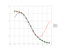
Unlike polynomial curve fitting (where a small section of a polynomial is forced to mimic a small section of data representing a sampling of physical data) the proper fit to the HD curve uses the equation that represents the underlying physics. It doesn't have to be bent to the task, it normally fulfills the task and fits the HD curve from 0 to infinite exposure.

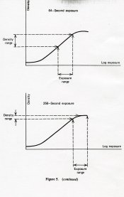
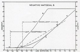
The correct function is not a bell curve. A bell curve (properly called a "normal distribution" or a "Gaussian distribution" http://en.wikipedia.org/wiki/Normal_distribution) does not fit an HD curve. As one is bell shaped and one is S shaped this is sort of obvious. Mangling the parameters of a bell curve so that half of it sort-of fits a portion of an HD curve is not the answer.

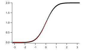
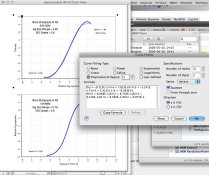
It is the integral (summation, adding together) of the bell curve distribution that needs to be used - it gives the total number of silver grains that have been exposed as a function of the light exposure. The integral of a probability is called a "Cumulative Distribution Function" (cdf), which in the case of a bell/normal/Gaussian distribution is the "Error Function" (erf). http://en.wikipedia.org/wiki/Error_function - please click on the link for the picture, it should look familiar...

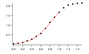
The following is a very crude simplification: The bell curve gives the probability that one more grains of silver will be exposed. In the toe region the probability increases with increasing amounts of exposure for rather obvious reasons: the more light shining on the film, the higher the chance a grain of silver will be activated. However, as the number of grains of exposed silver in the film increases the probability of light hitting an unexposed grain falls. After all the grains are exposed the probability of another grain getting exposed is zero (though, as we all know, probabilities never fall to zero, rather they become infinitely improbable).

So we have two sets of probabilities: one for the toe and one for the shoulder. There are several factors contributing to the physics at the toe region, but as a Gaussian function with a bit of a twiddle fits the data well enough it is what is commonly used for this part of the curve.

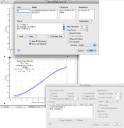
The integral of a Gaussian distribution - the “error function” or “erf” - can only be represented numerically. There is no closed form solution to the erf. Your math package may or may not include the erf even though it is a very common function in physics. An easy and universal method for calculating an HD curve is with a spread sheet and simple numerical integration. An Excel file is provided at http://nolindan.com/UsenetStuff/GaussianHD.xls

 

[Nicholas Lindan]

I don't really understand why we are trying to work with other curve fits if they don't fit as well and have to be patched.

They aren't patched. No more than the transition from ice to water is 'patched'.

The erf fits better than any other function: it fits the physics and it fits the data. Use a polynomial to fit an HD curve from the toe to 2x the exposure at the shoulder...

The man didn't get his picture on a 10-spot for nothing.

 

[Lee L]

Thanks for the spreadsheet and explanations Nicholas.

Lee

 

[Nicholas Lindan]

With all this being said, there is a place for making a polynomial approximation to an HD/erf curve and that is when a simplified model will do adequately. For all practical photographic purposes a polynomial approximation will be more than adequate if only a section of the HD curve is needed.

A polynomial (except for 0 and 1st order) can not fit a straight line. As an HD curve has a straight line section and two straight line asymptotes, using one polynomial for the entire thing is impossible.

To fit the entire curve with polynomials will take 5 separate polynomials: three 1st order polynomials (lines) for the asymptotes and straight line section; and two 5th order polynomials for the toe and shoulder joins, at the join points the first and second derivatives are continuous. The entire specification would only take 4 (x, y) points: the toe zero-slope point (which also specifies dmin); the two end points of the straight line section; and the shoulder zero-slope point (which also specifies dmax).

 

[RalphLambrecht]

... Use a polynomial to fit an HD curve from the toe to 2x the exposure at the shoulder...

Nicholas

Please elaborate.

 

[RalphLambrecht]

... A polynomial (except for 0 and 1st order) can not fit a straight line. As an HD curve has a straight line section and two straight line asymptotes, using one polynomial for the entire thing is impossible.

To fit the entire curve with polynomials will take 5 separate polynomials...

I think it can. Take a look at the attached example. Same data as before, curve-fit with a 4th-order polynominal. A 6th-order poly makes an even better fit, but even this example works well for toe and the straight-line midsection.

 

[Nicholas Lindan]

Please elaborate.

Try to use a polynomial to fit the blue HD curve in http://nolindan.com/UsenetStuff/GaussianHD.xls as shown in the graph over the range of X values from 5.5 to 7.5; for extra fun try to fit the red curve. The data is in c8..c88 for the x values, i8..i88 for the blue density curve and f8..f99 for the red derivative of the density dD/dE curve.