I guess I’ll just have to scan the wedge and use one of the tools that work off the scanned image (or just measure the densities in PS?)
It doesn't really matter what kind of data you start out with; it can be the L-component from Lab* samples, or logD reflected density, whichever you have at hand. You can even start with an RGB reading (or any of its components). It helps if you're comparing apples to apples, at least in order not to get too confused in the process. When doing this manually/with Excel, I tend to work with L from Lab* because I can easily get that on both input and output (through a photospectrometer reading, but a scanned or photographed photo and the sample tool in Photoshop/GIMP would work as well).
When taking the readings in Excel, I normalize them by defining the lightest reading as L=100 and the darkest reading as L=0, then adjust all the values in-between to that scale.
I find it also really helps to make a scatter plot of the data to get a feeling for what the adjustment curve needs to be.
For instance, I did this the other day for a Van Dyke digital negative linearization because a friend needed some inkjet negatives for this process. Here's the data I acquired, which I then inverted and normalized:
| L-value of original digital step wedge |
L-value measured on printed sample |
Normalized, inverted L-value |
| 100 |
34.77 |
0.0 |
| 95.8 |
35.72 |
1.6 |
| 91.3 |
36.18 |
2.4 |
| 86.7 |
36.99 |
3.8 |
| 82 |
36.41 |
2.8 |
| 77.7 |
35.91 |
1.9 |
| 72.9 |
37.46 |
4.5 |
| 68.1 |
35.78 |
1.7 |
| 63.2 |
38.25 |
5.9 |
| 58.6 |
39.07 |
7.3 |
| 53.6 |
39.68 |
8.3 |
| 48.4 |
42.43 |
12.9 |
| 43.2 |
44.84 |
17.0 |
| 37.8 |
48.25 |
22.8 |
| 32.7 |
52.09 |
29.3 |
| 27.1 |
57.22 |
37.9 |
| 21.2 |
65.26 |
51.5 |
| 15.2 |
75.3 |
68.5 |
| 9.3 |
84.46 |
84.0 |
| 3.6 |
91.97 |
96.7 |
| 0 |
93.94 |
100.0 |
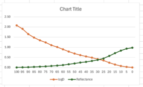
These are the plotted data (scatter plot):
The blue line is the measured, normalized L-value (Y axis) against the input, original L-value (X axis).
The orange line is a smoothed out, idealized version of this curve that ignores the noise that resulted from real-world imperfections. There's a bit of a fudge-factor going on here, as you can see.
The green line is basically the orange line, but with the X and Y axes swapped. This is the correction curve that I used in GIMP (or Photoshop etc.) Note that this correction curve does the linearization as well as the inversion to a negative in one go.
I then made a test print with the compensation curve, measured and plotted it:
As you can see, it's not perfect. At this stage, I could have either modified the adjustment curve, or added a second adjustment curve on top of it to fine-tune the result (this is what Calvin Grier describes in his linearization manual). I admit I did neither and just printed the darn negatives already; these were intended for kallitypes and I know the photographer would be toning his prints, and playing with them in the darkroom anyway, so I figured that trying to linearize the negatives to perfection for my materials (paper, sensitizer, light source) and workflow would not be of much added value. YMMV.
Hope this helps - and note that while the above looks simple enough, in practice, it always confuses the heck out of me whenever I go about re-inventing this particular wheel one more time (which I virtually always end up doing for some reason). There's merit to the collection of linearization tools/processes out there (Precision Digital Negatives, Easy Digital Negatives, Grier's Calibration series, etc.), especially if you want to have a proven, well-documented workflow that you can follow step by step.