Methodology and Curve Interpretation

End Table

A
End Table

  • 1
  • 1
  • 73
Cafe Art

A
Cafe Art

  • 8
  • 3
  • 197
Sciuridae

A
Sciuridae

  • 6
  • 3
  • 193
Takatoriyama

D
Takatoriyama

  • 6
  • 3
  • 179

Recent Classifieds

Forum statistics

Threads
197,660
Messages
2,762,589
Members
99,432
Latest member
sciencegirl100
Recent bookmarks
0

aparat

Member
Joined
Sep 5, 2007
Messages
1,177
Location
Saint Paul,
Format
35mm
So which curve in each are you applying ΔX to?
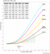
Personally, I am not using ΔX, but I programmed the option in so the user can decide whether to use it or not. Currently, it can be applied to any curve individually or all in the family. It can also be applied to curves that are not in the family, but can be predicted to be part of the family, such as LSLR=2.2, SBR=7, Ḡ=0.62, etc. It can be useful to see how different curve shapes, toes, slopes affect the interplay among parameters, such as CI, Gamma, ΔX, ΔD, etc. I am still trying to figure out the best way to present the data so that the plots do not appear too busy, esp. on mobile devices with limited screen real estate. I still have a lot of work to do. It will be months before I have anything to show.

One other thing that I think can be useful to photographers is seeing how particular curves of interest, such as for a "normal" scene luminance or "normal" in the sense of CI, fit into the family of curves. Here, my program synthesized two extra curves, as an example, one, marked "L7" and one marked "ISO." By coincidence, the L7 and the 2.5 minute curves coincide (sorry about the pun), except that the 2.5 minute curve is actual, whereas the "L7" curve is synthetic. Nevertheless, they share the same values of all the parameters of interest and the same overall tonality. This is possible because of the statistical model of the characteristic curve used here. It fits the data quite well. The ISO curve was generated the same way. The synthetic curves are plotted with dotted lines.
ferraniaP30FamilyWithExtras.png
 
OP
OP
Stephen Benskin
Joined
Jan 7, 2005
Messages
2,603
Location
Los Angeles
Format
4x5 Format
Personally, I am not using ΔX, but I programmed the option in so the user can decide whether to use it or not. Currently, it can be applied to any curve individually or all in the family. It can also be applied to curves that are not in the family, but can be predicted to be part of the family, such as LSLR=2.2, SBR=7, Ḡ=0.62, etc. It can be useful to see how different curve shapes, toes, slopes affect the interplay among parameters, such as CI, Gamma, ΔX, ΔD, etc. I am still trying to figure out the best way to present the data so that the plots do not appear too busy, esp. on mobile devices with limited screen real estate. I still have a lot of work to do. It will be months before I have anything to show.

One other thing that I think can be useful to photographers is seeing how particular curves of interest, such as for a "normal" scene luminance or "normal" in the sense of CI, fit into the family of curves. Here, my program synthesized two extra curves, as an example, one, marked "L7" and one marked "ISO." By coincidence, the L7 and the 2.5 minute curves coincide (sorry about the pun), except that the 2.5 minute curve is actual, whereas the "L7" curve is synthetic. Nevertheless, they share the same values of all the parameters of interest and the same overall tonality. This is possible because of the statistical model of the characteristic curve used here. It fits the data quite well. The ISO curve was generated the same way. The synthetic curves are plotted with dotted lines.

View attachment 326296

Just wondering because you have a curve family and are showing two speed points without indicating which curve they are from. With the two points off on their own and not readily associated with any specific curve, it appears that you have one speed per curve family which can't be the case. Also, ΔX appears to fall the same distance from the speed point to its right in all three examples and since ΔX's relationship to the fix density point of 0.10 is dependent on ΔD, and if they are from curves with the same ΔD, they should have the same speed difference. If the curve used fits the ISO parameters then the two points should have the same speed. Small point, neither should be labelled as ISO.
 

aparat

Member
Joined
Sep 5, 2007
Messages
1,177
Location
Saint Paul,
Format
35mm
Just wondering because you have a curve family and are showing two speed points without indicating which curve they are from. With the two points off on their own and not readily associated with any specific curve, it appears that you have one speed per curve family which can't be the case. Also, ΔX appears to fall the same distance from the speed point to its right in all three examples and since ΔX's relationship to the fix density point of 0.10 is dependent on ΔD, and if they are from curves with the same ΔD, they should have the same speed difference. If the curve used fits the ISO parameters then the two points should have the same speed. Small point, neither should be labelled as ISO.
Sorry. I misunderstood your question. I thought you were asking me for my preference. Generally, I try not to express a personal preference. Instead, I try to incorporate broad functionality into the program so that the user can decide what they prefer.

Since we are talking about technicalities, let me try to address your question. The relationship between ΔX and ΔD is not exact, so it will not produce identical results, even for curves that have been found to have approximately the same ΔD. It's not that ΔX mathematically depends on ΔD, but, rather, Nelson and Simmonds (1955) identified an inverse relationship based on empirical data. In the paper, they derived their ΔX equation from a simple least-squares "parabolic" fit of the data from previous and current studies, so, by definition, it is an approximation. They used a graphical calculator to obtain their approximate ΔX speed values. Moreover, they used a mathematical model of the characteristic curve based on what they refer to as the "Luther" equation (e.g., the graphical calculator in Fig 11 is based on that model). That equation fits only curves with a toe and straight-line portion (like the one in blue my post #9 above), so that adds another layer of variability. In the end, when applied to real data, all of the computed parameters are approximations, and that's what I tried to show above. The differences, in the case of ΔX, are very small, but, when used to compute film speed, they will be slightly different from family to family. For example, for the "ISO" curve (Δlog-E=1.3, ΔD=0.8, 0.1 over B+F), ΔX may be 0.28987, or it may be 0.29604, or it may be exactly 0.29, and that's what I tried to show. And, on my end, the curve itself is an approximation, with only 21 actual data points and the rest being interpolated based on my model of the characteristic curve. I agree that I should have made it more clear.

Regarding this statement: "it appears that you have one speed per curve family which can't be the case," I don't understand what you mean. I show the "ISO" curve (dotted line), which is generated to comply with the ISO standard for film speed measurement. That is the speed for the family, and the arrow points to the log exposure value used to calculate that speed. If you look at the table in the left-upper corner, you see that each curve has its own Effective Film Speed (EFS), so each curve has its own speed. Is that what you mean?
 
OP
OP
Stephen Benskin
Joined
Jan 7, 2005
Messages
2,603
Location
Los Angeles
Format
4x5 Format
Sorry. I misunderstood your question. I thought you were asking me for my preference. Generally, I try not to express a personal preference. Instead, I try to incorporate broad functionality into the program so that the user can decide what they prefer.

Since we are talking about technicalities, let me try to address your question. The relationship between ΔX and ΔD is not exact, so it will not produce identical results, even for curves that have been found to have approximately the same ΔD. It's not that ΔX mathematically depends on ΔD, but, rather, Nelson and Simmonds (1955) identified an inverse relationship based on empirical data. In the paper, they derived their ΔX equation from a simple least-squares "parabolic" fit of the data from previous and current studies, so, by definition, it is an approximation. They used a graphical calculator to obtain their approximate ΔX speed values. Moreover, they used a mathematical model of the characteristic curve based on what they refer to as the "Luther" equation (e.g., the graphical calculator in Fig 11 is based on that model). That equation fits only curves with a toe and straight-line portion (like the one in blue my post #9 above), so that adds another layer of variability. In the end, when applied to real data, all of the computed parameters are approximations, and that's what I tried to show above. The differences, in the case of ΔX, are very small, but, when used to compute film speed, they will be slightly different from family to family. For example, for the "ISO" curve (Δlog-E=1.3, ΔD=0.8, 0.1 over B+F), ΔX may be 0.28987, or it may be 0.29604, or it may be exactly 0.29, and that's what I tried to show. And, on my end, the curve itself is an approximation, with only 21 actual data points and the rest being interpolated based on my model of the characteristic curve. I agree that I should have made it more clear.

Regarding this statement: "it appears that you have one speed per curve family which can't be the case," I don't understand what you mean. I show the "ISO" curve (dotted line), which is generated to comply with the ISO standard for film speed measurement. That is the speed for the family, and the arrow points to the log exposure value used to calculate that speed. If you look at the table in the left-upper corner, you see that each curve has its own Effective Film Speed (EFS), so each curve has its own speed. Is that what you mean?
You do know I wrote a paper on Delta-X. My comments had to do with the way information is presented on your curve and that I was confused so I asked a question, but if you tend to get this defensive over an inquiry that could help improve your app then I'll just pass in the future. Just a couple of points.

Speed for a family of curves is a new one on me. What I was asking was which curve the ΔX speed was for. As all the curves can have ΔX speeds, and it's suggested to only use ΔX when the contrast is different than the ISO parameter, I don't see the confusion. The ΔX speed was sitting at the bottom of the graph by itself and it wasn't apparent which curve it represented. Perhaps connecting the points to the film curve or maybe including them in the table in the left-upper corner would make it clearer.

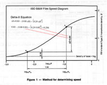
I'm sure you're aware the ISO parameters is a graphical version of the Delta-X equation. If you were deriving your values for speeds from the 0.10 fixed density and ΔX using a real or mathematical model that matched the ISO parameter, then the speeds would be effectively identical. The ISO contrast parameter is basically a short cut for determining Delta-X speeds. For those not aware, ΔX, like the fractional gradient speed, uses a constant in it's speed calculation. It's not simply the reciprocal of the exposure. How else can the fractional gradient speeds be 2/3 to 1 stop slower than those from 0.10 when they are generally found for normal about a stop to the left on the film curve. Without the constant, the speeds would be one stop faster than those derived from 0.10. As 0.297 is the general value of ΔX for the ISO aim ΔD or 0.80, the constant needs to be one that adjusts for the Δlog-H difference. Just wasn't sure you were aware of this and you could have simple indicated what constant you used. Again, as it wasn't clear which curve the ΔX was representing, I simply asked the question as to which curve the results represented.

Fractional gradient speed from Safety Factors in Camera Exposures, CN Nelson.

1673334468987.png


ISO parameters with Delta-X equation
1673334169444.png


Relationship between ΔD and ΔX. The inverse relationship has to do with ΔX speed in relation to the fix density speed with changes in film gradient, ΔD. This is the very nature of fractional gradient and why the fixed density method's agreement with print speeds is not as strong.

1673334821940.png


If I'm not mistaken the "Luther" equation was used with W speed. It's been years and I never cared for W speed.

1673334026904.png


Without further derailing this thread, the reason why I started it was to explain the strengths and weaknesses of the various methods of determining contrast. To show the way something is measured can influence the results. I know I had just gotten started and then dropped it, but I believe it's an important topic that is often overlooked.
 

Attachments

  • 1673336315855.png
    1673336315855.png
    171.6 KB · Views: 81
  • 1673334263135.png
    1673334263135.png
    103 KB · Views: 81
Last edited:

ic-racer

Member
Joined
Feb 25, 2007
Messages
16,490
Location
USA
Format
Multi Format
Inertia is easy to find with a spreadsheet derived automated system because of the linear regression function almost all spreadsheets have. That is the only reason I use an inertia-based method (W). I found coding Delta-X and 0.3G on a spreadsheet difficult because there are no functions to derive those in my spreadsheet software.
One reason I post that complaint many times here is for someone to correct me and indicate "(fill in the blank) software will calculate that..." and this is essentially what is happening in this thread. Aparat has indicated the software will calculate those functions (Delta-X and 0.3G), which is great!

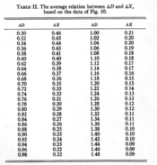
One stumbling block I came across trying to code this [Delta-X] in a spreadsheet is finding the Delta D automatically to solve the equation to generate the table Steve shows "Table II the average relation between Delta D and Delta X..."

Screen Shot 2023-01-10 at 8.39.22 AM.png


This is a typical example, but there is no easy way to get the spreadsheet to solve the polynomial to find the points that would be Delta D.
For example the first point needed to find Delta D would be Y = 0.1. So what is X if Y is described by the equation for the film curve below?
I can solve it 'myself' with it being about -2.51, but if I have to do it myself, I would be easier to use an plastic overlay on a printed version of the graph.

Screen Shot 2023-01-10 at 8.48.25 AM.png
 
Last edited:

aparat

Member
Joined
Sep 5, 2007
Messages
1,177
Location
Saint Paul,
Format
35mm
Inertia is easy to find with a spreadsheet derived automated system because of the linear regression function almost all spreadsheets have. That is the only reason I use an inertia-based method (W). I found coding Delta-X and 0.3G on a spreadsheet difficult because there are no functions to derive those in my spreadsheet software.
One reason I post that complaint many times here is for someone to correct me and indicate "(fill in the blank) software will calculate that..." and this is essentially what is happening in this thread. Aparat has indicated the software will calculate those functions (Delta-X and 0.3G), which is great!

One stumbling block I came across trying to code this [Delta-X] in a spreadsheet is finding the Delta D automatically to solve the equation to generate the table Steve shows "Table II the average relation between Delta D and Delta X..."

View attachment 326323

This is a typical example, but there is no easy way to get the spreadsheet to solve the polynomial to find the points that would be Delta D.
For example the first point needed to find Delta D would be Y = 0.1. So what is X if Y is described by the equation for the film curve below?
I can solve it 'myself' with it being about -2.51, but if I have to do it myself, I would be easier to use an plastic overlay on a printed version of the graph.

You are on the right track. If you're using a typical spreadsheet program (e.g., MS Excel), you can calculate Delta X by using the Table II from @Stephen Benskin post above and use it as a look-up table. You can use this equation: y=y1+ (x-x1)*(y2-y1)/(x2-x1) to get intermediate values of y from the look-up table. In fact, Nelson and Simmonds created the table for that very purpose. The method may strike you as crude, but it will give you a close-enough approximation.
 

aparat

Member
Joined
Sep 5, 2007
Messages
1,177
Location
Saint Paul,
Format
35mm
@Stephen Benskin I sincerely apologize if you found my post defensive. I apologized for misunderstanding your questions and tried to address them as accurately as I could to explain the discrepancy you thought was there. I don't know how else to address a question so as not to come across as defensive. English is not my first language so perhaps that is the source of my perceived tone.
 

Bill Burk

Subscriber
Joined
Feb 9, 2010
Messages
9,154
Format
4x5 Format
See if you can find the point with gradient 0.3 times the average.

Then illustrate where Delta-X and ISO estimate that point.

ISO will only find that point at its parameters within tolerance (about 0.62 Contrast Index), while Delta-X should fairly well estimate that point over much of the family of curves.
 
OP
OP
Stephen Benskin
Joined
Jan 7, 2005
Messages
2,603
Location
Los Angeles
Format
4x5 Format
@Stephen Benskin I sincerely apologize if you found my post defensive. I apologized for misunderstanding your questions and tried to address them as accurately as I could to explain the discrepancy you thought was there. I don't know how else to address a question so as not to come across as defensive. English is not my first language so perhaps that is the source of my perceived tone.

I over-reacted and also apologize. I was only making an observation that it wasn't obvious to me which curve the Delta speed values were referencing.
 
Last edited:

Bill Burk

Subscriber
Joined
Feb 9, 2010
Messages
9,154
Format
4x5 Format
I would like to see a dot for each curve’s Delta-X placement, or a range with ends labeled. I’d expect to see a tight grouping except at extremes.

When you look through Davis’s BTZS you see a lot of graphical evidence to suggest that you should change your EI for every change of development time. But I think a similar illustration showing Delta-X speeds would lead you to accept that you can settle on an EI for the film and leave it at that.
 

snusmumriken

Subscriber
Joined
Jul 22, 2021
Messages
2,370
Location
Salisbury, UK
Format
35mm
Inertia is easy to find with a spreadsheet derived automated system because of the linear regression function almost all spreadsheets have. That is the only reason I use an inertia-based method (W). I found coding Delta-X and 0.3G on a spreadsheet difficult because there are no functions to derive those in my spreadsheet software.
One reason I post that complaint many times here is for someone to correct me and indicate "(fill in the blank) software will calculate that..." and this is essentially what is happening in this thread. Aparat has indicated the software will calculate those functions (Delta-X and 0.3G), which is great!

One stumbling block I came across trying to code this [Delta-X] in a spreadsheet is finding the Delta D automatically to solve the equation to generate the table Steve shows "Table II the average relation between Delta D and Delta X..."

View attachment 326323

This is a typical example, but there is no easy way to get the spreadsheet to solve the polynomial to find the points that would be Delta D.
For example the first point needed to find Delta D would be Y = 0.1. So what is X if Y is described by the equation for the film curve below?
I can solve it 'myself' with it being about -2.51, but if I have to do it myself, I would be easier to use an plastic overlay on a printed version of the graph.
Forgive me if I have misunderstood the problem, but I think I would use Solver, which is built into Excel, to solve the equation (obtained by fitting a polynomial trendline and displaying the equation) for Delta X given Delta Y, or vice versa.

EDIT: Just seen @aparat's post #31 above, which crossed mine in the ether. My suggestion of using Solver is just a step advance on creating a look-up table.
 
Last edited:

ic-racer

Member
Joined
Feb 25, 2007
Messages
16,490
Location
USA
Format
Multi Format
Forgive me if I have misunderstood the problem, but I think I would use Solver, which is built into Excel, to solve the equation (obtained by fitting a polynomial trendline and displaying the equation) for Delta X given Delta Y, or vice versa.

EDIT: Just seen @aparat's post #31 above, which crossed mine in the ether. My suggestion of using Solver is just a step advance on creating a look-up table.

Yes, that [Solver] is how I got the -2.51. But aparat's program will not require that step from the user.
 

aparat

Member
Joined
Sep 5, 2007
Messages
1,177
Location
Saint Paul,
Format
35mm
Since we are talking about the characteristic curve and methodology, there is a very basic issue that can be potentially confusing and may even cause people to misinterpret the characteristic curve and some of the related parameters. The issue has to do with quantifying and displaying exposure values in the two-dimensional coordinate system. I have seen log exposure values presented in a number of different ways, making comparisons among curves from various sources tricky. Sometimes, authors do not even specify what sort of encoding or unit they use; they just say "log exposure" or something equally vague. Another issue has to do with the aspect ratio of the plot, which can skew one's perception of the overall shape of the characteristic curve. Yet another issue has to do with the limits and tick marks of the plot. It may seem like a simple matter of cosmetics, but I've seen people being confused by the lack of consistency in the literature. I admit I have found the lack of standardization a bit of a pain.

What are your preferences for displaying log exposure values and other aspects of plotting the characteristic curve?

Here are some examples:

Kodak's absolute log values in lux-seconds, using the mantissa-characteristic notation:


Kodak's absolute log values in lux-seconds:

Kodak's absolute log values in millilux-seconds:

Ilford's relative log exposure values in ascending order:

BTZS relative log values in descending order (related to the step tablet):

Todd and Zakia (1969) interval scale related to the steps of the step tablet:


With that in mind, I have implemented a few of those methods, giving the user the option to chose any method they like and to easily convert from one encoding to another, select their own plot limits, tick marks, aspect ratio, etc. Here are some examples:


Bill Burk

Subscriber
Joined
Feb 9, 2010
Messages
9,154
Format
4x5 Format
My favorite is square aspect ratio, medium lines at 0.10 log units, thick lines at 0.20 log units and thin lines at 0.02 log units. Points that are marked for the odd numbers fall between the thin lines. This makes it easy to plot and read 0.01 values.


Chuck_P

Subscriber
Joined
Feb 2, 2004
Messages
2,369
Location
Kentucky
Format
4x5 Format
What are your preferences for displaying log exposure values

Log exposure 0.0 through 3.0 from left to right with 0.1 interval tick marks. This makes the log exposure axis easier, for a simpleton like me, to interpret each zone. There's a fair amount of zone system talk related to all these type threads with all the very heavy heavy technical speak, ya know. I am going to assume most think of the horizontal axis in terms of the delineation of the zone scale, at least I do anyway. Since 0.3 is the log of 2 and every 0.3 interval on the log exposure scale is one stop and easily related to the exposure settings on the lens, it seems to me that is a consistent, more intuitive manner by which to display the horizontal axis......for most that are trying to utilize ZS principles. But maybe there is something I am completely getting wrong here, idk.
 
OP
OP
Stephen Benskin
Joined
Jan 7, 2005
Messages
2,603
Location
Los Angeles
Format
4x5 Format
Log exposure 0.0 through 3.0 from left to right with 0.1 interval tick marks. This makes the log exposure axis easier, for a simpleton like me, to interpret each zone. There's a fair amount of zone system talk related to all these type threads with all the very heavy heavy technical speak, ya know. I am going to assume most think of the horizontal axis in terms of the delineation of the zone scale, at least I do anyway. Since 0.3 is the log of 2 and every 0.3 interval on the log exposure scale is one stop and easily related to the exposure settings on the lens, it seems to me that is a consistent, more intuitive manner by which to display the horizontal axis......for most that are trying to utilize ZS principles. But maybe there is something I am completely getting wrong here, idk.

You're not wrong. They are all just different ways to communicate information. What's used all depends on the intended purpose and need.
 

Michel Hardy-Vallée

Membership Council
Subscriber
Joined
Apr 2, 2005
Messages
4,793
Location
Montréal, QC
Format
Multi Format
I've just started plotting H+D curves, so I used Excel and adjusted everything by hand, which is tedious.

I went with absolute logE in mililux-seconds because that way I was able to understand what I was doing, and relate correctly step tablet density values with exposure.

I used a square grid so that the two dimensions had the same scale. Major divisions at 0,3 logE and minor ones at 0,1 logE. That is enough resolution to find out the toe/straight line/shoulder portions by eye, but some computational help wouldn't hurt.

As an aside, in methodological terms, what I would find the most useful is a set of procedures/practices to ensure that I can relate in-camera exposure with step-tablet curves. So far, I have been winging it this way:

- contact-print a step tablet unto film, process, and measure
- do a series of exposures in-camera with the same film, same process, and measure
- If I get, for instance, a density of 0.94 with a 2.29 logE exposure from my step tablet, and a 0.94 density on my in-camera negative, then I can consider that both strips of film (processed identically) have received the same amount of light, i.e. 2.29 logE.
- That way I can relate f-stop/diaphragm combination to step-tablet values, and start thinking in terms of tonal reproduction.
 

ic-racer

Member
Joined
Feb 25, 2007
Messages
16,490
Location
USA
Format
Multi Format
If the x-axis is millilux-sec, then, besides you, only Steve or Bill could use it, because it would require a calibrated sensitometer.
My sensitometers are all calibrated to an "in house" standard I developed using film*. So the only speed analysis I can share here is a comparison of two films. This works fine for me, because even if my sensitometers were calibrated to the same traceable standard as yours, I'd still not use the information to set my camera in the field. I use in-camera test for that.

*Actually copied from Air Force Instruction 14-202; 28 March 1994

Screen Shot 2023-01-11 at 5.57.07 PM.png
 
Last edited:

Bill Burk

Subscriber
Joined
Feb 9, 2010
Messages
9,154
Format
4x5 Format
The relationship of ISO film speed and the MCS which hit the film at the speed point is absolute and straightforward.

See the top scale of this example from my EG&G chart template.

The top scale slides left to right over the graph you created by your own measurements.

Where I see 0.1 density on a curve which met ASA parameters, I tape the scale down aligning that point under the film nominal speed. I trust Kodak already did the work in the lab that guarantees that speed.

For my purposes I consider that close enough to take as a working calibration. I cannot claim absolute calibration but it is a good relative calibration.

 
OP
OP
Stephen Benskin
Joined
Jan 7, 2005
Messages
2,603
Location
Los Angeles
Format
4x5 Format
I've just started plotting H+D curves, so I used Excel and adjusted everything by hand, which is tedious.

I went with absolute logE in mililux-seconds because that way I was able to understand what I was doing, and relate correctly step tablet density values with exposure.

I used a square grid so that the two dimensions had the same scale. Major divisions at 0,3 logE and minor ones at 0,1 logE. That is enough resolution to find out the toe/straight line/shoulder portions by eye, but some computational help wouldn't hurt.

As an aside, in methodological terms, what I would find the most useful is a set of procedures/practices to ensure that I can relate in-camera exposure with step-tablet curves. So far, I have been winging it this way:

- contact-print a step tablet unto film, process, and measure
- do a series of exposures in-camera with the same film, same process, and measure
- If I get, for instance, a density of 0.94 with a 2.29 logE exposure from my step tablet, and a 0.94 density on my in-camera negative, then I can consider that both strips of film (processed identically) have received the same amount of light, i.e. 2.29 logE.
- That way I can relate f-stop/diaphragm combination to step-tablet values, and start thinking in terms of tonal reproduction.

You're not going to be able to quantify the exposure to any real degree of confidence. But you really don't need to. Use the characteristic curve to determine contrast and for tone reproduction. If you want an idea for camera exposure this might help. Hg is 10x Hm (speed point). Pick an EI that works for you and you can calculate and apply relative log-H. ie 0.8/125 = 0.0064 lxs. Hg = 10 * 0.0064 = 0.064 lxs at the metered exposure point.

Exposure for Sunny 16.jpg


1673486923533.png
 
Last edited:

Bill Burk

Subscriber
Joined
Feb 9, 2010
Messages
9,154
Format
4x5 Format
What Stephen shows is based on the ASA/ISO speed definitions like mine is.

He is providing “arithmetic lxs” while I use “Log mcs” *as shown on a calculator (top scale of the graph on post #45).

Note where he says the metered point is 10x the speed point. On Log or arithmetic scale that’s easy to do. Add 1 to Log scale, or move the decimal point one place in arithmetic scale.
 

aparat

Member
Joined
Sep 5, 2007
Messages
1,177
Location
Saint Paul,
Format
35mm
My favorite is square aspect ratio, medium lines at 0.10 log units, thick lines at 0.20 log units and thin lines at 0.02 log units. Points that are marked for the odd numbers fall between the thin lines. This makes it easy to plot and read 0.01 values.


Bill, I really like this idea! It has a kind of understated elegance while being very easy to read. I have been working on something like that. It's a responsive plot that changes grid lines and tick marks depending on the degree of zoom. Otherwise, all these primary, secondary, and tertiary lines would look pretty bad zoomed all the way out, esp. on a small screen. But, zoomed in, they can be fully visible. These days, all browsers and mobile devices support resolution-independent vector graphics.

Do you keep the data points visible along the curve or do you display the line without the points?
 

Bill Burk

Subscriber
Joined
Feb 9, 2010
Messages
9,154
Format
4x5 Format
I laser print with all the lines and draw graphs by hand on them. So the lines are always there.

I also appreciate when people share the underlying data.

The mark vi graph is hard to see, but I drew green lines on the step wedge calibration actual values. When I draw my own graphs, the x-axis values are always on a green line.
 

aparat

Member
Joined
Sep 5, 2007
Messages
1,177
Location
Saint Paul,
Format
35mm
I think this falls under the general umbrella of methodology and the characteristic curve analysis. I found some interesting looking curves in Kodak's PDF document F-4001, which concerns the T-MAX P3200 film. On page 8, the characteristic curves appear to be wrong. I am attaching them here. They seem to be more for an ISO 100 film, rather than the ISO 1000-1200 that the P3200 appears to be. Another small issue is the very low B+F density, which appears to be significantly lower than the current 135 version of the film. This is not a big deal, but I thought it was interesting. I wonder if this was just an innocent mistake, and, if so, how it ended up in the wrong document.
 

Attachments

  • F4001.pdf
    365.6 KB · Views: 87
Photrio.com contains affiliate links to products. We may receive a commission for purchases made through these links.
To read our full affiliate disclosure statement please click Here.

PHOTRIO PARTNERS EQUALLY FUNDING OUR COMMUNITY:


Ilford ADOX Freestyle Photographic Stearman Press Weldon Color Lab Blue Moon Camera & Machine
Top Bottom