I swore I would stay out of this thread ...
When fitting a mathematical function to a physical process one should use a function that is derived from the physics of the process. If that is not possible one should use the simplest representation that gives an adequate numerical result.
Fitting polynomials to data points - splining - originated with naval architecture. A spline is simply a bent stick
http://en.wikipedia.org/wiki/Flat_spline used to generate a curve for drawing the shape of a ship’s hull. The spline stick was held in place by ‘knots’ or ‘dog’ weights. Spline interpolation, formalized by Newton, uses a series of polynomials to represent the curve of the spline stick given the position of the knots - thus allowing the computation of a smooth ship’s hull to an arbitrary precision using rather crude data as the input. The technique has expanded to any application where intermediate data points are required. The most common mathematical splines are cubic functions that fit 4 points or 3 points and a first derivative - only the curve between the inner points is used as the generated curve. A curve of n knots is represented by n - 1 seperate polynomial functions, each with four coefficients; it is hardly a data reduction technique. The same technique can be used to generate a set of polynomials that have continuous second derivatives at the knots - useful in the design of roller coasters and cams where smooth acceleration is required.
Spline interpolation is very common simply because it is convenient. It will generate a well behaved curve through any arbitrary set of data points. The technique is heavily used in computer aided mechanical design and computer generated graphics. However, there are no physical processes that follow a splined function and thus the technique is frowned upon for modeling natural phenomenon.
It is possible to take the spline concept further and generate higher order polynomials and ratios of polynomials in an attempt to fit one equation to a complete set of data points. The results are often unsatisfactory as the function is not well behaved at the ends of the data set and the higher derivatives of the function are ‘bumpy’
http://en.wikipedia.org/wiki/Runge's_phenomenon . The somewhat sophomoric approach of fitting, say, a 9th order polynomial to 10 data points also suffers from the amplification of measurement noise that is inevitable when determining the data points.
Least-squares curve fitting is the correct method of determining function coefficients that model a data set
http://en.wikipedia.org/wiki/Least_squares . A least-squares curve will not go through the data points like a set of splined polynomials will. However, this can often be a blessing as the curve will smooth out the noise of the measurements used to generate the data set. The least squares method is not limited to polynomials and can be used to find the coefficients for any arbitrary function. It is always a good idea to use a function that has something to do with the underlying physical process: polynomials for power-law relations; straight lines for linear relations; exponentials, logarithms and sines & cosines for differential equations.
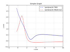
The physical processes that give rise to the HD curve are covered in chapter 5 of Meese, revised ed.. The three parts of the HD curve are due to different physical processes and therefore there is no one function that models the entire curve. Meese also points out that it is often easier to deal with the derivative (dD/dE) of the HD curve as the physical process of image formation gives rise to a function that gives the increase in density for an increase in exposure. The resulting function is integrated to give the HD curve.
The physics of image formation give rise to dD/dE equations of the same form as the normal ‘bell-curve’ Gaussian distribution function
http://en.wikipedia.org/wiki/Gaussian_function . It is possible to model the toe and the shoulder region as halves of the standard bell curve, each half having different parameters. Although Meese doesn’t go into it, the straight line joining the toe and shoulder of modern emulsions is adequately modeled with, of all things, a straight line.
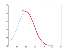
The result of integrating two 1/2 bell curves, one for the toe and one for the shoulder, with a straight line in between, is shown below.
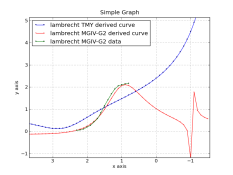
It is - relatively - easy to fit this set of three functions to a real-life HD curve.
As the function is derived from the physics of the exposure process it has few artifacts, is continuous for all derivatives, and is well behaved outside of the set of data points. The resulting function has an infinite toe and shoulder that quickly become asymptotic to dmin and dmax, even if only the inner portion of the HD curve is used for data points.
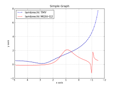
However one should keep in mind that most modern materials are made from more than one emulsion and it will require the summation of an HD curve for each emulsion to generate the HD curve of the paper or film. This can be seen clearly in the roller-coaster shape of the HD curve for a variable contrast paper. When one is faced with the decomposition of a material’s HD curve into the response of its individual layers/emulsions the job becomes a PITA and the resulting mathematical function a hideous over complication.
The simplest approach is to use the raw measurement data points as the definition of the HD curve and do a simple linear interpolation between the data points. This no-brainer method yeilds intermediate results that are within a few percent of the real curve - far more accurate than any shutter. And the method is completely immune from artifacts and malignant behavior between and outside of the data points.
Using curve fitting to find a ‘Personal EI’ (PEI) is, IMO, a waste of time. One’s PEI is almost always equal to a -1/3 of a stop adjustment to manufacturer’s speed rating. This is because the methodology for finding a PEI is different from the manufacturer’s method for determining ISO. People are happier using a PEI for negative work because it helps to hide errors in exposure determination - where it is always wise to err on the side of overexposure. After 100 years of refinement the best advice is still ‘Expose for the shadows, develop for the highlights’ and keep as much of the image as possible on the straight portion of the HD curve. It is in printing that the shape of the HD curve becomes important.
In the old days students were required to shoot Kodachrome to prove their ability to properly determine exposure, exposing B&W was considered too much of a cake-walk. To aid in this effort, camera manufacturers calibrated metering systems not to any ASA/ISO standard but to give the best results when shooting slides. Matrix Metering is designed for exposing color slides, which is why it sometimes gives sub-optimal results for negative materials as it's prime directive is "Don't blow the highlights". Usually, setting the camera’s control dial to ‘A’ gives the best results with slides, bracketing if the lighting is tricky.
All this curve fitting is best left to an MS thesis; when taking pictures it leads to paralysis by analysis.