Comparative reciprocity failure of available sheet films

[gainer]

BTW, my method fits just about any reciprocity curve, but my observation that the correction for any film is a factor of tm^1.62 is limited to those films that believe in it. The factor happens to be the amount of correction required at 1 second of metered time. Any time anyone gets some additional experimental data, my equation and its assumptions can be tested. For instance, if you find that a particular film needs 200 seconds when the metered exposure is 100, the amount of correction is 100, and that is Af*(100^1.62), so Af*1738 = 100 and Af = .056. After a few such results, you can average AF and see how that average fits the trials that went into calculating it.

 

[gainer]

Lee, the value of corrected time, 165 seconds, that I calculated for 120 seconds metered time was by using your linear fit. I had ASSumed that your linear fit was good from that point up. I then went to the previously posted data and used the values 1920 metered and 2288 corrected to calculate the value 0.001766 for the Af coefficient which I then used in the calculation tc = tm^1.62*0.001766+tm to calculate the following:
tm........tc...........te.......tpf
80........82.1........82........77.4
160......166.6.......166......161.9
240......252.7.......252......249.4
480......519.0.......519......522
960......1079.7.....1090.....1092.6
1920.....2288.9.....2288.....2286.7

te are the posted experimental values, tpf are the values I calculated by your power fit equation, tc= tm^1.06559*0.72538.

How on earth did you get correlations so close to 1.00000? I personally would rather see the mean square deviation.

 

[Lee L]

Pat,

The point I was making in posting the linear model for Acros was that there was very little difference in practice between working from the power or linear model with this film. The attached chart shows percentage error for each model over the range of the experiment that found any reciprocity correction necessary, i.e. above 120 seconds. The linear model is -6% to +5% and the power model from -2.5% to +0.58%. The power model and your model are obviously better fits, but the linear model is perfectly usable in practice.

I thought Andre's numbers looked familiar, and I found them at http://home.earthlink.net/~kitathome/LunarLight/moonlight_gallery/technique/reciprocity.htm where I'd seen them before. The page states that these numbers for Acros are preliminary, the third test roll that the author shot. He lays out his procedure there, and claims an accuracy of approximately 0.02 log density units with his Pentax spotmeter and a light table, and an ability to get within 1/15th of a stop in typical tests. However, the first three data points in his results, at adjustments for 80, 160, and 240 seconds, show variations of 5% or less from the base times. In other words, three of the six data points used for the curve fitting are below the accurate measurement threshold given by the author, so I don't see the point in belaboring a fit to marginal data.

You could find the author of CurveExpert and request that he change his choice of default quality of fit statistics. I wondered about that as well.

Lee

 

[ghost]

The formula should have lead you to these numbers:
The time to be added to 10 seconds indicated exposure for a film that has a correction of 0.3 seconds at 1 second indicated is:
tadd = 0.3*(10^1.62) = 12.51. .

Add 12.51 seconds to the indicated 10 seconds to get 22.5 seconds after correction for non-linear reciprocity. Your suspicion was correct. I don't know what you did to get 4 seconds instead of 12.5, but you surely didn't calculate 10^1.62 in the process!

Remember: the coefficient a in the equation is the amount of the reciprocity CORRECTION at the measured exposure time of 1 second, 0.3 seconds in the case at hand.

Thanks for the correction- I was simply using your chart to add numbers- it's obviously way more complicated than that.

I'm ashamed because I'm supposed to be a reasonably competent person (I do instruments and calibration for a living)...but this math is just way over my head for use in the field- Maybe someone somewhere has come up with a simple additive chart that I could understand.
It sure is neat to have exposure to scientific people of this caliber on a board of mostly us "artsy" types- I salute your superior grey matter fellas!- but I have no clue - how does one perform the function "^"?

 

[gainer]

Thanks for the correction- I was simply using your chart to add numbers- it's obviously way more complicated than that.

I'm ashamed because I'm supposed to be a reasonably competent person (I do instruments and calibration for a living)...but this math is just way over my head for use in the field- Maybe someone somewhere has come up with a simple additive chart that I could understand.
It sure is neat to have exposure to scientific people of this caliber on a board of mostly us "artsy" types- I salute your superior grey matter fellas!- but I have no clue - how does one perform the function "^"?

The ^ symbol means "to the power of". It is not something one can do with paper and pencil unless the number on the right is an integer. Thus, 2^2 means 2 raised to the power of 2 which is simply 4, but 2^1.62 is not so easy. The TI30XIIS pocket calculator and many others have a key with that symbol. Using it, I find that 2^2=4 and 2^1.62=3.073750363. I am glad I didn't have to design the circuitry in that little light-powered pocket calculator. I is capable of math operations that I could not do at my desk during the 30 years of work at NACA-NASA without laborious calculation of power series on an electromechanical Friden or Marchant desk calculator.

We use our grey matter to pursue knowledge along paths which are mysteriously chosen from among many available ones. I consider myself lucky that others who have pursued other paths have shared the fruits of their pursuits, and am happy to be able to share what I have found along my path.

 

[Lee L]

I've been playing around with Bond's data a bit more today, and moved from Curve Expert to QtiPlot under linux (it's also freely available for Mac and MS Windows if you install the necessary QT environment on those platforms).

I've been looking at the consequences of adding the metered time to a log equation as Gainer does in his formula.

Covington notes that the Schwarzschild formula accommodates the approximate logarithmic character of reciprocity failure, but is a good fit only at longer exposures. So Covington modifies the formula as follows.

where t = time in seconds
and 'p' is the Schwarzschild exponent, which varies between about 0.50 and 1.00, with 1.00 being perfect reciprocity.

Schwarzschild
actual speed = rated speed * t^(p-1)

Covington
actual speed = rated speed * (t+1)^(p-1)

When this equation is manipulated to produce adjusted exposure times, one gets

corrected time = (metered time +1)^(1/p)-1

In the same way, Gainer's formula , where 'a' is a coefficient dependent on film type,

corrected time = metered time ^ 1.62 * a + metered time

is a better fit than the straight log fit because it makes the correction relative to the initial value.

Gainer's formula can be rewritten as

y=a*x^b+x

where 'b' is a constant with a value of 1.62
and 'a' is a variable coefficient, dependent on the film behavior

compare this to a straight log fit

y=a*x^b

where 'a' is a variable coefficient
and 'b' is a variable exponent

Taking the cue from Covington and Gainer, one can add the value of x (which is the metered exposure time) to the straight log fit as follows

y=a*x^b+x

or

corrected time in seconds = a * metered time ^ b + metered time

The only difference between this model and Gainer's is that 'b' becomes a variable exponent rather than a constant exponent equal to 1.62, and this equation can be plugged into a curve fitting program like QtiPlot and regressed. So this is just a more generalized form of Gainer's equation to accommodate films that might not "believe in" Gainer's constant (as Pat puts it) for the exponent. BTW, it hasn't been mentioned in this thread, but that constant is also known as phi, the golden ratio, and is also the ratio in the Fibonacci series and many natural phenomena.

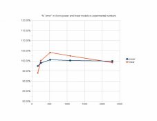
Making the Gainer adjustment (adding in the metered time) to a standard log fit generally makes for a better fit to the Bond data, especially with time exposures at the shorter end of the spectrum.

Doing just that with QtiPlot produces the following values when regressing Bond's data using the formula y=a*x^b+x All values but one hit within +/- 20% of Bond's data. TMY is actually a somewhat better fit to a straight log function. (R^2 and Chi^2 values are shown, but one must keep in mind that tweaking to optimize R^2 with data containing sufficient randomness can lead to silly numbers. See http://www.statisticalengineering.com/r-squared.htm )

===========================================
Bond Data Modified Power fits using QtiPlot

using function: y=a*x^b+x
where: y = adjusted time in seconds
x = metered time in seconds

TMX
a = 0.040427011642017
b = 1.7298680795766
Chi^2/doF = 3.5603085938797e+00
R^2 = 9.9995145162988e-01

TMY
a = 0.18601192358624
b = 1.3478556218539
Chi^2/doF = 1.9330084508589e+00
R^2 = 9.9994757744607e-01

100 Delta
a = 0.056981442009898
b = 1.5754970970282
Chi^2/doF = 2.4755726666553e+00
R^2 = 9.9993698631413e-01

HP5+
a = 0.029331463486986
b = 1.8845746981645
Chi^2/doF = 1.8558446352135e+02
R^2 = 9.9883106078538e-01

Tri-X
a = 0.20711252730778
b = 1.5186636391859
Chi^2/doF = 9.3638439358780e+01
R^2 = 9.9936933497974e-01
=============================================
I'll attach a revised .pdf with the modified log regressions from Bond's data. You can easily build your own chart in a spreadsheet using your own data and regressions.

For those without much spreadsheet experience, the following functions are standard in spreadsheets and flat ascii representations of formulae:

the carat ^ in y^x means "raised to the power", y raised to the power of x
the asterisk * is a multiplier, e.g. 3*2=6 This is to avoid confusion between any variable 'x' and the common handwritten "x" as a multiplier.
Don't include spaces in your spreadsheet formula. I've only done that in this post for human readability.

If you can't afford MS Office, openoffice.org has a completely free office suite that runs natively in linux, under MS Windows, and the new version 3.0 is now native on the Mac OS-X. openoffice will also create .pdf files.

Lee

P.S. After posting I went back and calculated the average value of the exponent b in the regressions of Bond's data using the modified power equation.
It's 1.61113

 

[gainer]

What you did is essentially the process I used: finding the best fit for each film to Bond's data and averaging the exponent of all the films. I plotted the resulting individual curves (the exponential part) on log-log paper. Sometimes the visual experience is more meaningful than the mathematical. The scatter about a straight line when 1.62 (or 1.61 for that matter) was used for all the films tested was as aceptable as the scatter about the optimum line for each film. The conclusion may thus be drawn that the average exponent obtained from all the films might have been obtained for rach film if enough repetitions of experiments were available. You may find as much scatter when a number of experienced photographers measure the lighting of the same scene. Each one may yet get a satisfactory negative.

 

[ghost]

Is there anyway this could be put into a nice little Excel workbook where you plug in your metered exposure and out pops the corrected exposure? Or am I dreaming here? You could win the APUG Nobel prize and be heroes with such a product...I forsee fame, endorsment deals, talk shows, ...groupies...

 

[Lee L]

Is there anyway this could be put into a nice little Excel workbook where you plug in your metered exposure and out pops the corrected exposure? Or am I dreaming here? You could win the APUG Nobel prize and be heroes with such a product...I forsee fame, endorsment deals, talk shows, ...groupies...

The chart attached to post #32 in this thread does that in 1/3 stop increments for the films with Bond data.

You could do your own spreadsheet with the Bond data and information already posted, but you'd need to test reciprocity for other films that you might want to include.

You could use Gainer's approach and use a pocket calculator with his formula and a list of films and appropriate coefficients.

If you want to regress data that you have or get from someone else against a given formula, you could download CurveExpert for MS Windows, or QtiPlot for Win, Mac, or linux. Several good formulae are in this thread for the copying.

Are you asking if you could do the regressions in Excel?

Lee

 

[gainer]

As a matter of curiosity, I was trying to find where I had used the magic number in a report. I thought I had mentioned it in "LIRF is Lurking at YOUR F-Stop". Any way, it involves the square root of 5. Using the theorem of Pythagoras and a compass and straight edge, one can construct a line that is the square root of 5 time the length of whatever length you set the compass for. You can, of course, construct the perpendicular to a line and lay off 2 units one the line and one length on the perpendicular. The line forming the right triangle with those two sides has a hypotenuse = square root of 5. Use the compass and straight edge to add one unit to an end of that hypotenuse. Bisect the resulting line and each part is of length 1.618... units.

 

[ghost]

The chart attached to post #32 in this thread does that in 1/3 stop increments for the films with Bond data.

You could do your own spreadsheet with the Bond data and information already posted, but you'd need to test reciprocity for other films that you might want to include.

You could use Gainer's approach and use a pocket calculator with his formula and a list of films and appropriate coefficients.

If you want to regress data that you have or get from someone else against a given formula, you could download CurveExpert for MS Windows, or QtiPlot for Win, Mac, or linux. Several good formulae are in this thread for the copying.

Are you asking if you could do the regressions in Excel?

Lee

dude- you guys are so far over my head....but yes- this chart is awesome- now...how do I use it- are the numbers under each film time corrected exposures (mm:ss?), OR adders, or multiplyers to get corrected exposure? this is an awesome tool- thanks in advance

 

[Lee L]

dude- you guys are so far over my head....but yes- this chart is awesome- now...how do I use it- are the numbers under each film time corrected exposures (mm:ss?), OR adders, or multiplyers to get corrected exposure? this is an awesome tool- thanks in advance

The times under the films are corrected times in mmm:ss (minutes: seconds) They are corrected from the metered times in seconds in the first column. The tinted times are the full stop numbers shown most often on light meters. The mmm:ss format for the corrected times is used to make it easier than converting hundreds or thousands of seconds to minutes. No adjustment of the corrected mmm:ss times is necessary, use as read. The data up to 240 seconds metered is within Bond's experimental range. Times adjusted from longer than 240 seconds metered are extrapolated beyond the experimental data.

The latest version I posted uses the more generalized form of Gainer's power formula, where his constant 1.62 is made a variable, and regressed from the data Bond found for those films.

Lee

 

[gainer]

A basic requirement of any equation describing reciprocity characteristics, it seems to me, is that it's constants for any given film should allow for a fairly general reciprocity curve. An equation that attempts to do so by the form:

tc = a*tm^b

does not meet that requirement. In fact, if the meter reading is assumed to be an inaccurate analog of the film's response, it would be more reasonable to say that the corrected meter response is tm + tc which then more closely matches the film's response. The the basic equation becomes:

tc = tm + a*tm^b

Now there are many more possibilities. One is that the constant b may in fact be a constant for all films and yet each film may require a different value of a.

 

[johnnywalker]

Tom,
About 5 yrs ago, I queried Ilford regarding the same reciprocity curves for their films. FWIW, here is an edited excerpt from their response:
We do use the same curve for ALL our films and it is essentially an average curve designed to be a reasonable guide for all our films. We are conscious that this is a weakness in our current Technical Information and we intend to provide curves for individual films when time and resources permit. However, there will be some batch to batch variability in this characteristic and so careful workers will need to run their own tests.

I asked basically the same question on the Ilford website some months ago, and the eventual answer coming back from their technical people was simply that they "stood by their curves". After reading all of this I'm getting a little annoyed at their simplistic and misleading answer to me.

 

[ghost]

Thanks for all your hard work on this guys, I will be using the chart for my long exposures moving forward- I'll let you know how it works out.

 

[Tom Kershaw]

If you have a pocket calculator such as the T1-30XIIS, you need only know 1 number for each film you use and one constant, 1.62, that is good for all films. The sequence of entries is as follows, where Af is the film constant, tm is the metered time, and tc is the corrected time.

tm^1.62*Af+tm = tc

Let's say that your film requires 0.5 seconds correction at tm=1 second. For that film, Af = 0.5. Now you're out shooting lumps of coal at in the deep woods (a common, though not often photographed, sight in West Virginia) and your meter tells you it will take 100 seconds. (Wish I had such a meter.). You whip out your TI30 and do:

100^1.62*.5+100 and the answer is 20424.9 seconds. But suppose you have another film with Af = 0.1. then:

100^1.62*.1+100 = 273.8

Patrick,

Is there any advantage to the TI30X compared to any other scientific calculator one might own? I see from the specifications that the TI30X has an equation recall function but as this is a short equation I assume a adhesive label on the back of the calculator would sufficient.

Tom.



Tom.

 

[gainer]

Patrick,

Is there any advantage to the TI30X compared to any other scientific calculator one might own? I see from the specifications that the TI30X has an equation recall function but as this is a short equation I assume a adhesive label on the back of the calculator would sufficient.

Tom.



Tom.

It just happened to be the one I found at my local drugstore that would do those functions. There is now a TI-30XIIS which I bought when I mislaid the other. More streamlined looking but otherwise about the same. Handy to have around in any case.