Average Gradient Methods

Diner

A
Diner

  • 1
  • 0
  • 43
Gulf Nonox

A
Gulf Nonox

  • 5
  • 2
  • 46
Druidstone

A
Druidstone

  • 7
  • 3
  • 99
On The Mound.

A
On The Mound.

  • 1
  • 0
  • 58
Ancient Camphor

D
Ancient Camphor

  • 6
  • 1
  • 68

Forum statistics

Threads
197,801
Messages
2,764,672
Members
99,478
Latest member
BS Taylor
Recent bookmarks
0
Joined
Jan 7, 2005
Messages
2,603
Location
Los Angeles
Format
4x5 Format
Average gradient can be a helpful tool. A single number describes the contrast of the film processed at a specific time and how it will respond to exposure. It is a description of the film's exposure input to density output. A collection of these gradient values obtained from a few development tests can be applied again and again to any photographic process, from traditional silver and platinum printing to digital scanning and printing. All that is required is to determine the conditions how the film is to be used, and plug it into a simple equation. Then find the processing time from the film test that produced the required gradient and you’re good to go. There is no need to do further film tests if there is a change the printing or shooting conditions. All that is required is recalculate.

There are a number of different techniques and variations used to find a film’s average gradient. The three principle methods are Gamma, Average Gradient or G Bar, and Contrast Index. The attached article, “Contrast Measurement of Black and White Materials,” and the attached paper, “Contrast Index,” discuss the different methods as well as their strengths and weaknesses.

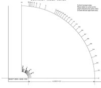
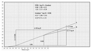
Gamma uses the straight line portion of the film. Fuji and Agfa use Gamma. Ilford’s Average Gradient, sometimes written as a capital G with a bar over it, measures 1.50 log-H units from 0.10 Fb+f. And Kodak’s CI uses two arcs 2.0 log-H units apart (see attachment).

What it all comes down to is which method produces the best results in the greatest number of situations with the greatest number of film types. As each method is an average of the film's gradient, how it averages is key. What part of the film curve should and shouldn’t be measured. For example, would the gradient obtained from measuring the curve from the lowest point on the toe to high up into the shoulder produce an accurate picture of the film because it is representative of the whole range of the film curve or would measuring an area that isn’t going to be used in most shooting situations produce unrealistic results?

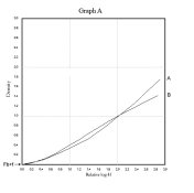
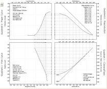
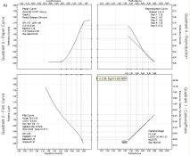
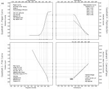
The attached Graph A is of two film curves – a long toed curve (A) and a medium toed curve (B). The point where each of the films is measured will produce a different value. My programs use two different methods automatically and has an option for a third. According to a variation of the Contrast Index method that I use, the two curves in Graph A have identical CIs.

Graph B shows a number of the different methods, including the Zone System’s Negative Density Range method.

So what would be the best method and why? Is there one? Does each method work equally well at different levels of contrast? What are the factors that must be considered?
 

Attachments

  • Contrast Measurement of Black and White Negativre Materials a.pdf
    418.2 KB · Views: 627
  • Contrast Index a.pdf
    926.1 KB · Views: 281
  • Contrast Index Meter.jpg
    Contrast Index Meter.jpg
    25.2 KB · Views: 258
  • Gradient Example A.jpg
    Gradient Example A.jpg
    58.1 KB · Views: 231
  • Gradient example B.jpg
    Gradient example B.jpg
    71.5 KB · Views: 261

Bill Burk

Subscriber
Joined
Feb 9, 2010
Messages
9,158
Format
4x5 Format
I use the Contrast Index meter on the left, printed on overhead material. I lay it on top of paper charts.

One advantage of this meter is the wide range of films accommodated without changing the setup of your test equipment.

At speeds of 400 or more, my thinnest densities are over 0.1 when I use the 10 ^ -2 exposure setting.

The left-hand arc hits part of the curve anyway, so I can get a reading almost all the time.

The other methods, if you have to have an 0.1 reading, will force you to adapt your equipment.
 

ffg

Member
Joined
Aug 12, 2011
Messages
10
Location
Hannover, Ge
Format
Multi Format
I would imagine that the best method is to not use these average gradient methods for a normal user who mostly uses one process. Better would be to just consider SBR as a function of dev. time as Phil Davis suggests. All the average gradient methods will produce errors in extreme situations, either by neglecting the toe characteristics or premature shouldering for low contrast negatives.
 
OP
OP
Stephen Benskin
Joined
Jan 7, 2005
Messages
2,603
Location
Los Angeles
Format
4x5 Format
Beyond the Zone System uses an average gradient method. As this thread is about the analysis the different methods, how does the BTSZ method work and what are its strengths? It's been awhile since I've read the BTZS specifics. I have a copy of the fourth edition open now.
 

ffg

Member
Joined
Aug 12, 2011
Messages
10
Location
Hannover, Ge
Format
Multi Format
in BTZS you start as always by determining your desired negative density range (DR) and find the appropriate subject brightness range (SBR) for your film curve. Usually you will convert the SBR to stops to facilitate your metering. Then as you gather data for many different dev. times for the same curve, you plot SBR as a function of dev. time. The strengths in this method are that you don't do any straight line fitting as you would when using the average gradient method for a priori given DR (according to some standards.) The obvious weakness is that this process is designed for one specific DR and if you work with vastly different printing methods, you have to analyze your core data more often. The average gradient methods (CI, G bar) are to my knowledge really designed for data-sheets etc. and not the individual user.
 

Bill Burk

Subscriber
Joined
Feb 9, 2010
Messages
9,158
Format
4x5 Format
I'll have to pay my library fines before I can check out BTZS again, but I recall it uses the same data set as I use now. Sensitometer exposed films developed at various intervals and read on a densitometer.

Then the Wonder Wheel or software determines the development time based on a paper (LER) and (SBR). Maybe Fred Newman can chime in but it's not that BTZS avoids using average gradient or CI... Just that it provides a practical interface to the user making it easy to apply the data in the field and in the darkroom.
 

ffg

Member
Joined
Aug 12, 2011
Messages
10
Location
Hannover, Ge
Format
Multi Format
I didn't really mentioning BTZS in my original post, and my point was not about metering technique, which BTZS really refers to. I was just saying that using average gradients for a common user is not the most accurate. Just to be clear BTZS does not really use average gradient. The disadvantage of average gradient method (whatever type) is that it is a straight line approximation of a much more complicated curve.
 
OP
OP
Stephen Benskin
Joined
Jan 7, 2005
Messages
2,603
Location
Los Angeles
Format
4x5 Format
Now that I know you aren't talking about a method specific to BTZS, I don't have to bone up on BTZS and can address the general concept. Basically, what you're talking about can be considered an average gradient method. You have rise and run. Just because you might decide not to calculate slope doesn't mean the principles or concerns are any different. Nor does it mean that you shouldn't be asking a few basic questions to confirm how well any technique works because no method is perfect. So, let me just state before going any further, pointing out any pros and cons of a methodology shouldn't be construed as an attack on any particular method or suggesting that any method is a failure.

For a short toed or medium toed curve, any average gradient method will work fine. Long toed films are another matter. How much and what parts of the curve to be measured need to be considered. Take Curve/Graph B from the examples in post #1. The method of using the desired density range and the subject luminance range would be like the Zone System example. For a seven stop subject luminance range, the Δlog-H is 2.10 logs to the right of 0.10 Fb+f. A line is drawn until it intersects with the film curve. The Δlog-H value is then divided into the density of the curve at this point minus 0.10 Fb+f to produce the average gradient for that film. In this example, the vertical line intersects the three curves at three different densities. This would indicate the three curves all have different average gradients. However, a different average gradient method concluded that two of the curves had the same average gradient value.

So, where the curve is measured is just as important with the density range method as any other. The density range can be a very accurate method if used properly. That means considering all the variables involved. In Curve/Graph B, there's an additional factor that needs to be considered for the method to reach its full potential. While the subject luminance range maybe 7 stops, the Δlog-H range isn't 2.10 logs. Camera flare reduces the illuminance range at the film plane. The testing method is flare free, which means an adjustment to the Δlog-H range is require to make the Δlog-H range of the test conform to the type of range encounter in use. For the Curve/graph B example, with a 1 1/3 stop flare factor, that would mean measuring not for a Δ2.10, but for a Δ1.70. At this point, Curve A and C have the same NDR.

This is basically the third method I use with the programs. It's a good method when doing detailed analysis. I've found that with short to medium toed curves, the projected negative density ranges using the other average gradient methods is spot on with the negative density range method. The disadvantage of the negative density range method is any log-H range adjustments when working with curve families using the more realistic variable flare models (the amount of flare changes with the luminance range, so the steps between each log-H reading won't be consistent).
 

ffg

Member
Joined
Aug 12, 2011
Messages
10
Location
Hannover, Ge
Format
Multi Format
You are right, these methods are totally equivalent because you can specify the NDR you want to calculate the average gradient with. These are just two numbers which are the inverse of each other. There is no approximation involved and hence you are using the data, you have worked hard to produce, to it's fullest. However, when you use some standards others have created, for instance average gradient with a specific NDR not connected to your process or CI, you *may* be making inaccurate assumptions about the film curve. The same film curve you have in front of you and really don't need to make any assumptions about. I hope you understand what I mean.

I must admit that I didn't read your previous post "zone system placement" in full detail, but I have a question about the flare. Do you add the flare (fixed or practical model) to the film curves before you analyze them or do you compensate afterwards?

Second question, how do you use your average gradient numbers in practice (in the studio or in the field) ?
 
OP
OP
Stephen Benskin
Joined
Jan 7, 2005
Messages
2,603
Location
Los Angeles
Format
4x5 Format
We seem to be in agreement.

I must admit that I didn't read your previous post "zone system placement" in full detail, but I have a question about the flare. Do you add the flare (fixed or practical model) to the film curves before you analyze them or do you compensate afterwards?

Flare isn't part of the determination of the average gradient of a particular film curve. The flare models are a way to determine the average gradient value to process the film to. For example, an average grade 2 LER for a diffusion enlarger is 1.05 (rise). The average scene luminance range is 2.20 (run) minus 0.40 flare for a run of (2.2-.40=1.8). 1.05/1.80 = 0.58. After processing your family of curves, determining their average gradients, and plotting those values on a Time/Gradient curve, you simple find the time for 0.58. If you decide to print on a condenser enlarger instead, you just change the rise/LER value to what you've got in your personal paper test (0.95 average grade 2 with condenser), plug it in to the equation, then find the processing time on the Time/Gradient curve. The gradients of the film haven't changed and you don't have to retest the film. Only the aim gradients have changed.

For the pluses and minuses, you add or subtract 0.30 for each stop change from the scene's luminance range:e.g. 1.30 = +3, 1.60 = +2, 1.90 = +1, 2.20 = N, 2.50 = -1, 2.80 = -2, 3.10 = -3.

Second question, how do you use your average gradient numbers in practice (in the studio or in the field) ?

The negative is the intermediary step between the subject and print. The gradient tells you how the luminance range will translate into the density range. As this is done with processing, average gradient is used in the darkroom. However, you still decide how the film is going to be processed in the field, N, N+1, etc. It's when you get back to the darkroom that N becomes CI 0.58 and according to the Time/CI curve example for Tri-X in Xtol that means a processing time of 6:15. For a condenser enlarger, N becomes, 0.95 / (2.2-0.40) = 0.52 and the processing time becomes 5:30.
 

Attachments

  • Tri-X, Time CI curve.jpg
    Tri-X, Time CI curve.jpg
    41.4 KB · Views: 139
OP
OP
Stephen Benskin
Joined
Jan 7, 2005
Messages
2,603
Location
Los Angeles
Format
4x5 Format
Okay, what about the very concept of average gradient? How many threads are about whether a film is more or less contrasty in developer A or developer B?

If everyone used average gradient, this wouldn't be a question. As long as the film's average gradients match, they have the same contrast and will produce identical prints (excluding local contrast differences). If people did a simple test that defines the film contrast, a huge amount of the threads here wouldn't exist, as well as a few photographic urban myths. Say good-bye to the question of films being inherently contrasty, say so long to magic developers, and say arrivederci to vague music analogizes to explain what to expect from a film/developer combination.:smile:

I have a saying, "contrast is contrast." While the saying may not be sweeping the country, it is never-the-less true. If properly determined, a gradient of 0.58 means the same thing no matter the film type.
 
Last edited by a moderator:

Bill Burk

Subscriber
Joined
Feb 9, 2010
Messages
9,158
Format
4x5 Format
.... As this is done with processing, average gradient is used in the darkroom. However, you still decide how the film is going to be processed in the field, N, N+1, etc. It's when you get back to the darkroom that N becomes CI 0.58 and according to the Time/CI curve example for Tri-X in Xtol that means a processing time of 6:15.....

What is funny is I was about to say. But I am not choosing 0.58 for N because I am choosing 1.00 LER.

I am also choosing 7 stops SBR.

Wait, it's 0.59

Again, arriving at the same number but for different reasons.
 

eclarke

Member
Joined
Jun 11, 2004
Messages
1,950
Location
New Berlin,
Format
ULarge Format
God, I'm not scientific enough..I look at the print, decide how I want to change it and make another until I like it (usually 3 or 4 sheets)...EC
 

ffg

Member
Joined
Aug 12, 2011
Messages
10
Location
Hannover, Ge
Format
Multi Format
Michael: This is what my discussion with Stephen was all about. The thing is that if you evaluate your average gradient with respect to those "extreme" points of the film curve you reach the same conclusion as looking at the curve itself. That is excluding local contrast. However you get in trouble when you try to generalize the analysis of normal situation to extreme situations, and this is the reason I don't like to use average gradients at all (here I mean the average slope of the function over a certain region.)
 
OP
OP
Stephen Benskin
Joined
Jan 7, 2005
Messages
2,603
Location
Los Angeles
Format
4x5 Format
Questioning the range of accuracy of a method is what this thread is about. Does the specific gradient method include the entire area of the curve that will be used in the field while excluding the areas of the curve that aren’t? This generally means matching the log-H range of the curve to the luminance range of the scene photographed.

I just don’t think it’s fair to use extreme examples for which the method isn’t even designed. Most of the situations photographers run into fall within a rather narrow range (see the Normal distribution Curve). Ninety-five percent all scenes fall within a 2 1/2 stop range of the average luminance or in other words from -2 ½ to + 2 ½. Sixty-eight percent fall within a 1 ¼ stop range of average luminance. It seems to me that the broader the test parameters, the higher the rate of potential error. It makes sense that any method would want to restrict the testing parameters as much as realistically possible. This means keeping them as close to the type of situations encountered most.

Aside from the way Davis decided to compensate for flare in the test, I believe his method is perhaps the best for the individual. He uses the NDR to define the height of the triangle (rise), and the log-H range for the base (run). It maybe best for the individual, but not in general.

A major purpose of any method is communication, and that includes the method in which the test was made. Placing “ISO” in front a film speed means that the standard’s very specific procedures have been followed. Anyone familiar with the standard understands how the film was tested. As is the same with the various average gradient methods.

This is the main reason why the Davis method works extremely well for individual use but not as well for general usage. For that to happen, there would have to be average gradient values for each potential value of the NDR for each curve. A good average gradient method needs to reflect specific shooting conditions yet not be too specific to be relevant for the gradient value to be used as a general reference.

I believe Contrast Index does that. Davis mischaracterizes CI as always measuring “a fixed portion of curve length, their values are unrelated to subject range.” The reality is quite the opposite. The key is the arc. As the “Contrast Index” paper states, “ as the log exposure range of the normally used part of the curve decreases, the average gradient, density range, and minimum and maximum densities increase.” In other words, as the arc increases, it covers a progressively smaller log-H range, so it tends to measure the part of the film curve the would normally be involved in the exposure at a given subject luminance range.

Now, average gradient isn’t a panacea and using it doesn’t mean everything is going to print effort free. But it will get you close enough the first time out. The graph example shows TX and HP5P both developed to a CI 0.61. I didn’t have to look hard for the two film examples either. I just went through my database looking for two films with the same CI. It appears that a simple numerical value can describe a curve quite well for the average conditions expected to be covered.

What about those situations that fall outside the intended parameters? What do you do for those really long luminance ranges? Just change the parameters. With something like CI, use a bigger arc. But for the really extreme situations, the Davis NDR version can be very effective. The graph attachment with the extended curve shows how this works. In Curve A the 1.05 NDR intersect the curve at Δ 2.98 log-H (10 Stops) for an average G of 0.35. Curve B extension illustrates a slight shouldering off. With this curve 1.05 NDR doesn’t intersect the curve until Δ3.75 log-H (12.5 stops) for an average G of 0.29.

Check it out and see how closely the numbers work out. Pick a LSLR and plug it into this equation:

CI * LSLR = NDR

See how closely the NDR on the curve matches the projected NDR from the equation.

Film is the intermediate step between the contrast of the subject and placing it onto the contrast of the paper. Processing the film can be thought of as a black box approach. We know what goes into the camera (luminance range + flare) and we know what comes out of the processed negative (density). By comparing the output to the input, we get a picture of what is going on with the processing.

Whether you use a quantifiable approach with step tablets and curves or a more instinctive hit and miss approach, the objective is the same. The goal is to define what the processing has done to the film in order to have greater control over the materials used in our art.
 

Attachments

  • Normal Distribution Curve.jpg
    Normal Distribution Curve.jpg
    77.5 KB · Views: 157
  • TX 0.61.jpg
    TX 0.61.jpg
    179.7 KB · Views: 128
  • delta 0.35.jpg
    delta 0.35.jpg
    264.3 KB · Views: 122

Bill Burk

Subscriber
Joined
Feb 9, 2010
Messages
9,158
Format
4x5 Format
A point I think Michael R 1974 is making is that some photographers seek out the far-beyond-average scene. For example looking out from the interior of a beach cave. A point you made in an earlier post Stephen, that if you use a highly active developer the toe doesn't get a chance to "come up to speed". These two examples are not well served by CI and are scenarios where the shape of the curve is significant to the results.

The straight photography on graded silver gelatin paper that I do is well-served by the CI model, it is great to see that less exposure range is used as less is relevant to the final print. And I just thought it was a convenient shape for the graph. Well, I knew the arc measured less exposure range as the CI went up, just didn't know it was deliberate.
 
OP
OP
Stephen Benskin
Joined
Jan 7, 2005
Messages
2,603
Location
Los Angeles
Format
4x5 Format
Bill, it was the whole concept of average gradient that was in question. I believe I showed how those can be handled. It's all about contrast. But if not an average contrast method of some kind than what other option is there to use? If not, then what?
 

Bill Burk

Subscriber
Joined
Feb 9, 2010
Messages
9,158
Format
4x5 Format
You did. It's brilliant. When shooting extremely long-range subjects it is a great idea to match the points chosen so they are more relevant to the part of the scale that you use.

Michael only hinted at applications where the shape makes a difference. There are some unresolved threads about the application of staining developers and multigrade papers. It's possible that it might take more than an average gradient to deal with the contrast in that application.
 
OP
OP
Stephen Benskin
Joined
Jan 7, 2005
Messages
2,603
Location
Los Angeles
Format
4x5 Format
There's an often repeated mantra, "open up 1/2 stop, and reduce development by 20%." I've attached a CI / Time Curve showing seven curve families. Four of the curves are from two films developed in two different developers. Good rule of thumb?
 

Attachments

  • Six Films, CI Time Curve.jpg
    Six Films, CI Time Curve.jpg
    65.6 KB · Views: 172

Bill Burk

Subscriber
Joined
Feb 9, 2010
Messages
9,158
Format
4x5 Format
I can use CI to fit subject brightness ranges to negative density range. I want my negatives to have a range approximately 1.0

Michael, your extended-range chart tells me right away that CI would be OK to model Acros, but if you need to use the part of the curve above XI you need to be aware of the shoulder.

To the open 1/2 stop and develop 20% less, I don't know what that would accomplish. It would produce a shorter-range negative with better shadows. If the negative would otherwise be too "contrasty", the action would kick the contrast down "about a grade" but it's not very accurate.
 
OP
OP
Stephen Benskin
Joined
Jan 7, 2005
Messages
2,603
Location
Los Angeles
Format
4x5 Format
I've already explained how no method encompasses all situations nor should they. The basic CI method accurately covers 95% of conditions faced.

Curve shape is a good question. This is the argument made in the Contrast Index paper. Gamma only uses the straight-line portion of the curve, which is not only difficult to determine in some cases, but also doesn't entirely represent the portion of the curve in usage. The paper doesn't cover shoulders though. The Theory of the Photographic Process does note that "the gradient of the characteristic curve is of such importance, especially in connection with the problems of tone reproduction, that it is often desirable to use a derivative curve...This graphic form is useful when it is desired to determine precisely the exposure value corresponding to some particular slope of the D-log E curve...for many purposes it presents the data in more convenient form and gives a more vivid mental picture of the relation between gradient and exposure."

Should variations in the upper end affect the overall average? According to tone reproduction theory, the perception of a quality print allows for compression of the shadows and highlights, but requires the midtones to be over a gradient of ~1.11 of that of the original subject. Tone reproduction theory also states that there isn't a perfect correlation between the negative density range and paper LER. According to Loyd Jones, "for the soft papers, the density scales of the negative (NDR) should in most cases exceed the sensitometric exposure scale of the paper (LER) (see Tone Reproduction Curve attachment). According to Theory of the Photographic Process, "For scenes having unusually long log luminance ranges (2.5 to 3.0), the tone reproduction curves for the first-choice prints were slightly to the left of the curve shown (in the example)...The gradient in the middletone region was always greater than 1.00 (usually 1.10 - 1.20) for the preferred prints of all scenes studied." So, there are no absolutes. A perfect match isn't necessary. Average gradient is a tool to describe how the subject is generally translated into density.

If you measure the entire range from the example, you get (top to bottom) 0.51, 0.41, 0.39. Which in a fixed flare developmental model is from -1 to -3. However, if you measure only up to where the two bottom curves begin to shoulder off at Zone X, you get 0.48, 0.47, 0.45, or -1 1/2 to -2. Then there is the question of flare. Flare for an average scene is around 1 to 1 1/3 stops. Flare's rule of thumb is that flare increases by 1/3 stop per stop increase in the luminance range. A fourteen stop luminance range could have around 3 stops of flare. This would mean measuring the density range of the curves at Zone XI instead of Zone XIV. Which one would best translate into a quality print? Good question. I don't test for such extremes. I don't even know if there is a paper that has a LER of 2.14 from the Acros curve. If there is, what would happen to the all important midtone contrast? I've attached a four quadrant reproduction curve with a ten stop luminance range and two stops flare. The film has a CI 0.43 and the NDR closely matches the paper's LER. Also, there's an example with a slightly higher paper grade. With the higher contrast, the midtone reproduction gradient has just reached 1.00.

These are all interesting questions. In extreme situations, does measuring the entire effective log-H range produce more desirable prints or does limiting the range of measurement in some way work best?

Whatever the answer, it doesn't negate the effectiveness of any of the average gradient methods in most situations generally encountered.
 

Attachments

  • Quad 4 - Tone Reproduction Curve.jpg
    Quad 4 - Tone Reproduction Curve.jpg
    20.1 KB · Views: 85
  • 10 stop luminance range.jpg
    10 stop luminance range.jpg
    85.4 KB · Views: 87
  • 10 stop luminance range higher paper grade.jpg
    10 stop luminance range higher paper grade.jpg
    83.8 KB · Views: 117

Bill Burk

Subscriber
Joined
Feb 9, 2010
Messages
9,158
Format
4x5 Format
what is the range? From darkest to lightest scene lumincance? Or from darkest to lightest to fit the paper (assuming no print manipulation)?

I'm starting to enjoy the "fact" that when you have anywhere from enough to too much range in a negative, it can make a nice print on Grade 2. And when you have almost no range and a very thin negative, Grade 3 will re-create the mood that led to that situation in the first place.
 
OP
OP
Stephen Benskin
Joined
Jan 7, 2005
Messages
2,603
Location
Los Angeles
Format
4x5 Format
Bill, you might find this interesting. Below are a number of four quads. The example #1 is considered normal. The reproduction curve, quad 4, should be to the left of the reference line which represents the original scene. If the print tones equal the original scene's, the print will appear dark and would require twice the viewing illumination as what was in the original scene. For a print to be considered of high quality, the midtones should have a gradient at least 1.0, but best over 1.10.

Example #2 has the same shooting conditions as the first. The negative was under developed and printed on a higher grade of paper to compensate. Notice how the higher tones in the reproduction curve are lighter and at a slightly lower gradient. The midtones and lower tones are at a higher gradient than in the first example.

Example #3 has a short luminance range. The negative CI has been increase to compensate and it is matched to a grade 2 paper. The fourth example also has a short luminance range, but the negative as processed normal and printed on a higher grade of paper. Interestingly, there is little difference in the reproduction curve.
 

Attachments

  • Normal Dev.jpg
    Normal Dev.jpg
    244.7 KB · Views: 93
  • Under Dev.jpg
    Under Dev.jpg
    247.4 KB · Views: 94
  • Short Luminance range - NDR match 2.jpg
    Short Luminance range - NDR match 2.jpg
    234.5 KB · Views: 76
  • Short Luminance range - LER match 2.jpg
    Short Luminance range - LER match 2.jpg
    230.3 KB · Views: 107
Photrio.com contains affiliate links to products. We may receive a commission for purchases made through these links.
To read our full affiliate disclosure statement please click Here.

PHOTRIO PARTNERS EQUALLY FUNDING OUR COMMUNITY:


Ilford ADOX Freestyle Photographic Stearman Press Weldon Color Lab Blue Moon Camera & Machine
Top Bottom