


dpgoldenberg
Member
- Joined
- Feb 18, 2009
- Messages
- 50
- Format
- Med. Format RF
Hi,
Over the past year or so, there have been at least two long threads here on the topic of plotting characteristic curves and fitting smooth functions to them. I have been playing with something along these lines, and I thought that there might be some interest in it. I am posting this in the hopes that someone might find it useful (or amusing) or might have some suggestions. I'll try to keep it fairly short, but would be happy to answer questions.
My idea is to fit the measured densities to a relatively simple mathematical function with a small number of parameters. After a bit of playing around I found this function:
D(x) = a1*ln(1+exp(a2*x + a3))
where D is density, x is exposure (on a logarithmic scale) and a1,a2, a3 are constants. ln is the natural logarithm and exp is the number e raised to the power in the parentheses.
The basic features of this function are that it begins at zero with zero slope, and the slope increases monotonically to a limiting value. It can thus describe the toe and linear region of a characteristic curve, but it is not suitable for a shoulder. My sense is that most modern films don't have much of a shoulder, and the toe and linear regions are, in any case, the important parts for assessing speed and contrast.
So far as I know, the equation and the parameters don't have any physical significance, but they are related to the shape of the curve in convenient ways:
1. The limiting slope of the linear region is a1*a2. If the exposure values are plotted as log base 10 values, this gives gamma. If (as I prefer) the values are plotted as log base 2, gamma is calculated as a1*a2/log10(2).
2. A fractional gradient (fg) can be defined as the gradient at any point divided by the limiting slope. This can be calculated as:
fg= 1/(1+exp(-a2*x - a3))
and can be solved for x to determine the exposure for a given fractional gradient:
x = (ln(f/(1-f))-a3)/a2
This can be used to calculate a speed point based on a defined fractional gradient (e.g. 0.3 or 0.5)
3. If the position of the toe is defined as the point where the fractional gradient is 0.5, this point is where:
x = -a3/a2
4. The width of the toe can be defined as distance between x values where fg = 0.1 and 0.9 (other values could be used, of course):
w = 2*ln(9)/a2
5. The equation for density can also be solved for x to give the exposure for a given density:
x = (ln(exp(D/a1) - 1)-a3)/a2
This can be used to calculate a speed point based on a minum density (e.g. 0.1)
The potential value of all of this is, I think, that it provides a fairly objective way of analyzing data and deriving parameters.
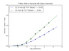
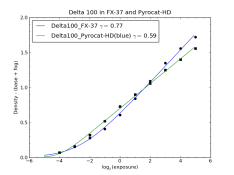
So far I have implemented this scheme in a Python script, using publicly available modules for the most of the math and plotting. I am attaching a sample plot, for TMY-2 developed in Pyrocat HD. In addition to the plot, the program outputs the following information:
15 min @ 73 F (blue)
gamma = 0.64 +/- 0.02
toe width = 2.55 +/- 0.76 stops
Exposure index set from density threshold (Zone I density = 0.10):
Speed point = -2.67 +/- 0.14 (log2exposure)
Corrected EI = 159.31 +/- 15.23
Avg. gradient (log10) = 0.60 +/- 0.02
Zone I density = 0.10
Zone V density = 0.81
Zone VIII density = 1.38
Exposure index set from fractional gradient (gradient = 0.30 * gamma):
Speed point = -3.38 +/- 0.12 (log2exposure)
Corrected EI = 260.80 +/- 20.89
Avg. gradient (log10) = 0.55 +/- 0.02
Zone I density = 0.04
Zone V density = 0.67
Zone VIII density = 1.25
The data for these curves were measured from camera exposures. My usual practice is to define log2(exp) = 0 as the exposure indicated by the meter. The program takes the EI used for the meter measurement, and calculates corrected EI values using defined values for fractional gradient or density threshold (Zone I density). It then calculates densities for Zone I, V and VIII based on the corrected EI.
I hope that this will be of interest to those with a weakness for the more geeky end of photography! In its present form, the program is not particularly user-friendly, but I am happy to share it. If there is substantial interest, I may also be willing to put in a bit more time to make it friendlier.
David
Over the past year or so, there have been at least two long threads here on the topic of plotting characteristic curves and fitting smooth functions to them. I have been playing with something along these lines, and I thought that there might be some interest in it. I am posting this in the hopes that someone might find it useful (or amusing) or might have some suggestions. I'll try to keep it fairly short, but would be happy to answer questions.
My idea is to fit the measured densities to a relatively simple mathematical function with a small number of parameters. After a bit of playing around I found this function:
D(x) = a1*ln(1+exp(a2*x + a3))
where D is density, x is exposure (on a logarithmic scale) and a1,a2, a3 are constants. ln is the natural logarithm and exp is the number e raised to the power in the parentheses.
The basic features of this function are that it begins at zero with zero slope, and the slope increases monotonically to a limiting value. It can thus describe the toe and linear region of a characteristic curve, but it is not suitable for a shoulder. My sense is that most modern films don't have much of a shoulder, and the toe and linear regions are, in any case, the important parts for assessing speed and contrast.
So far as I know, the equation and the parameters don't have any physical significance, but they are related to the shape of the curve in convenient ways:
1. The limiting slope of the linear region is a1*a2. If the exposure values are plotted as log base 10 values, this gives gamma. If (as I prefer) the values are plotted as log base 2, gamma is calculated as a1*a2/log10(2).
2. A fractional gradient (fg) can be defined as the gradient at any point divided by the limiting slope. This can be calculated as:
fg= 1/(1+exp(-a2*x - a3))
and can be solved for x to determine the exposure for a given fractional gradient:
x = (ln(f/(1-f))-a3)/a2
This can be used to calculate a speed point based on a defined fractional gradient (e.g. 0.3 or 0.5)
3. If the position of the toe is defined as the point where the fractional gradient is 0.5, this point is where:
x = -a3/a2
4. The width of the toe can be defined as distance between x values where fg = 0.1 and 0.9 (other values could be used, of course):
w = 2*ln(9)/a2
5. The equation for density can also be solved for x to give the exposure for a given density:
x = (ln(exp(D/a1) - 1)-a3)/a2
This can be used to calculate a speed point based on a minum density (e.g. 0.1)
The potential value of all of this is, I think, that it provides a fairly objective way of analyzing data and deriving parameters.
So far I have implemented this scheme in a Python script, using publicly available modules for the most of the math and plotting. I am attaching a sample plot, for TMY-2 developed in Pyrocat HD. In addition to the plot, the program outputs the following information:
15 min @ 73 F (blue)
gamma = 0.64 +/- 0.02
toe width = 2.55 +/- 0.76 stops
Exposure index set from density threshold (Zone I density = 0.10):
Speed point = -2.67 +/- 0.14 (log2exposure)
Corrected EI = 159.31 +/- 15.23
Avg. gradient (log10) = 0.60 +/- 0.02
Zone I density = 0.10
Zone V density = 0.81
Zone VIII density = 1.38
Exposure index set from fractional gradient (gradient = 0.30 * gamma):
Speed point = -3.38 +/- 0.12 (log2exposure)
Corrected EI = 260.80 +/- 20.89
Avg. gradient (log10) = 0.55 +/- 0.02
Zone I density = 0.04
Zone V density = 0.67
Zone VIII density = 1.25
The data for these curves were measured from camera exposures. My usual practice is to define log2(exp) = 0 as the exposure indicated by the meter. The program takes the EI used for the meter measurement, and calculates corrected EI values using defined values for fractional gradient or density threshold (Zone I density). It then calculates densities for Zone I, V and VIII based on the corrected EI.
I hope that this will be of interest to those with a weakness for the more geeky end of photography! In its present form, the program is not particularly user-friendly, but I am happy to share it. If there is substantial interest, I may also be willing to put in a bit more time to make it friendlier.
David