Curve fitting

[alanrockwood]

I have been experimenting with fitting curves for film testing. I think I have found some equations that do a pretty good job. They are not based of well established physical theory, but I believe they are based on some qualitatively reasonable physical concepts.

I will start with a simple equation designed to fit the toe and straight line part of the curve. Instead of working in log(exposure) and absorbance (i.e. density) coordinates I will work in linear exposure and transmission coordinates. (It is possible to transform the results to new variables in log(exposure) and absorbance.)

First, I assume that at zero exposure the transmission of developed film is some amount given by Fl, where Fl is defined as 10^Fg, where Fg is base plus fog in absorbance space. This simply converts base plus fog between absorbance space and transmission space.

Then I assume that the transmission as a function of exposure decreases asymptotically toward zero. (This assumption does not allow for a shoulder in log(exposure) and absorbance coordinates, but that problem can be fixed using a more elaborate fitting equation designed to handle this issue.)

As a first guess at an equation one might try

Tr=Fl/(1+Ex)

where Tr is the transmission (i.e. fraction of light passing through the film), Fl relates to base plus fog as described earlier, and Ex is the exposure.

This equation has some useful qualitative features, i.e. in log(exposure), absorbance space it has an asymptotic value equal to base plus fog as zero exposure, followed by a toe region, and then a linear region. However, it is not flexible enough because it does not allow one to place the toe, does not allow one to specify how abrupt the toe is, and does not allow one to match the slope of the linear region.

To allow one to place the toe one can modify the equation as follows.

Tr=Fl/(1+(Ex/Et)

Where Et controls where the toe is located on the exposure curve.

One can control the how gentle the transition is in the region of the toe and the slope in the linear region by introducing two more parameters, m and n as follows.

Tr=Fl/(1+(Ex/Et)^m)^n

By taking the limit as Ex approaches infinity one can show that the slope in log(Tr), absorbance space is controlled by m*n.

One can also show that when Ex/Et is small compared to 1 (i.e. in the deepest part of the toe region) curve is basically controlled by m*(Ex/Et)^n.

I won't go into the details of the math, but I believe that by using for parameters, Fl, Et, m, and n it is possible to provide a good fit to a typical exposure curve, i.e. one can fit base plus fog, the location of the transition region between base plus fog and linear, the slope of the linear region, and the abruptness or gentleness of the transition region.

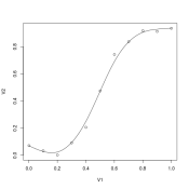
I have tried this on a limited amount of experimental data, and it seems to work pretty well.

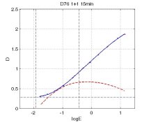
The weakness of this equation is that it results in infinite density at infinite exposure. Instead there is a straight line that goes to infinity. It is possible to make the equation more elaborate in order to introduce a shoulder, but I would go into that right now.

With modern software one can fit the equation to produce a continuous smooth curve that gives a good representation of the experimental curve, but the bumps and jags in the experimental data have been smoothed out. (By the way, this scheme should work much better than conventional smoothing algorithms.)

Any comments?

 

[bernard_L]

I understand what you want to achieve. But, the closed-form analytic expressions that you use have limitations: you point out the shoulder, but then you have the compensating film-dev combination with some sort of break of the slope around zone V, etc, etc... You soon find that you need a new equation for each different film.

What you need is called least-squares splines: piecewise cubic polynomials with continuous second derivatives, that are not constrained to pass exactly through the data, but to approximate them as best as possible (least squares). If interested, PM me, and I'll send you some matlab code that can easily be adapted to the free look-alikes Scilab or Octave.

 

[alanrockwood]

I understand what you want to achieve. But, the closed-form analytic expressions that you use have limitations: you point out the shoulder, but then you have the compensating film-dev combination with some sort of break of the slope around zone V, etc, etc... You soon find that you need a new equation for each different film.

What you need is called least-squares splines: piecewise cubic polynomials with continuous second derivatives, that are not constrained to pass exactly through the data, but to approximate them as best as possible (least squares). If interested, PM me, and I'll send you some matlab code that can easily be adapted to the free look-alikes Scilab or Octave.

Thanks for the reply.

When fitting curves (by the way, my discussion centers around fitting, not interpolation, so the fitted curve does not generally go through each point) there is generally a balancing between several factors. One is the flexibility of the fit function, and another is the "reasonableness" of the fitting function.

One of the strengths of using cubic splines for fits is that they are very flexible, i.e. they can fit most any function in some manner.

One of the weaknesses of splines is that they are very flexible, i.e. they can end up trying to chase the noise of the data.

Regarding the reasonableness of the fitting function, it is a big advantage if the fitting function of similar form to the underlying physical function. To take a simple example, if one were to fit the fluorescence intensity as a function of time after an impulse excitation it would be better to use an exponential function than a polynomial, because an exponential is a good fit to the underlying physical process, whereas a (globally-defined) polynomial is not. Spline functions tend to be somewhat intermediate in this respect.

Also, more parameters would be typically required to fit the data using splines than using the method I am discussing.

Anyway, after saying all that, I agree that the general approach I am suggesting will not give a good representation of strange bumps and jags in a curve, but it is also much more resistant to chasing noise.

However, I am interested in learning more about your approach. At one time I had Octave loaded on my computer, but I never became competent with it. I know a little more about R. I am not fully competent with R, but I am closer to competence in R than in Octave.

Most of the curve fitting I have done has used Psi-Plot, which actually has some pretty powerful methods for doing curve fitting, including a capability to use user-defined functions.

 

[bernard_L]

(...)the underlying physical function. To take a simple example, if one were to fit the fluorescence intensity as a function of time after an impulse excitation it would be better to use an exponential function(...)

Yes, in that case there is a simple physical process involved, and very good reason to fit an exponential; to the extent that if the exponential does not fit well, one should investigate and find why, rather than adding extra complexities in the fitting function.

The case of the D-logH curve is different. The underlying physics is complex: distribution of halide paricles sizes, all the alchemy of emulsion fabrication.

Also, more parameters would be typically required to fit the data using splines than using the method I am discussing.

Not so. Least-squares splines use a handful of real numbers, called "nodes"; they are the abscissas of points of transition between two polynomials; because the second-order derivative is continuous, they do not appear visually as "breaks". I typically place the first node about where I see the transition between toe and mid section, and another at the transition between mid and shoulder. Total: two real parameters. Well, actually, there are all the coefficients of the polynomials, but these are transparently taken care of for you by the fitting algorithm.

Take a look at: http://www.mathworks.com/matlabcentral/fileexchange/13812-splinefit , and you'll know as much as I do. As you can see on http://www.mathworks.com/matlabcentral/fileexchange/screenshots/6036/original.jpg , the least squares spline fit does not chase the noise. And being polynomial, it is easy to compute a derivative, normally problematic with noisy data.

 

[Photo Engineer]

At KRL we have an excellent fit to all film and paper curves using a cubic spline. IDK the equation, as it has been years since I had to even look at it. It was converted to computer code and the computers did all of the work for us.

PE

 

[dasBlute]

if you know a little R, you can use a smoothing spline.

say you have your input points in a file called 'curve.xy.txt':
0.00000000 0.07171922
0.10000000 0.03320194
0.200000000 0.001970976
0.30000000 0.09175587
0.4000000 0.2059855
0.5000000 0.4742702
0.6000000 0.7423032
0.7000000 0.8366679
0.8000000 0.9174252
0.9000000 0.9118453
1.0000000 0.9352661

you could then load the data, fit a curve, and plot it thus:

### R code from here... ###

# read the data
xy = read.table('curve.xy.txt',header=FALSE)
nrows = dim(xy)[1]

# optional: generate a vector of weights, this lets us tell
# the smoothing function to pay more attention to the endpoints
# yw = [10 1 1 1 1 1 1 1 1 1 10]
yw=c(10,rep(1,nrows-2),10)

# generate the smoothed function
# spar = is the smoothing parameter, bigger is smoother
# df = degrees of freedom, 3 is cubic, plenty smooth
# w = vector of weights [if you want]
s = smooth.spline(xy,spar=0.4,df=3,w=yw)

# sample the smoothed function at a finer resolution than the input
ys = predict(s,seq(0,1,0.01))

# plot the data and overlay the smoothing spline on top
plot(xy,xlim=c(0,1),ylim=c(0,1))
lines(ys)

View attachment 108108

 

[wombat2go]

Also,
There is an old OpenOffice spreadsheet from the time before OpenOffice had built in polynomial classes.

It is called CorelPoly.ods originally by Laurent Godard and modified
Can still be obtained from here : http://extensions.libreoffice.org/extension-center/improved-trend-lines

I used this quite a lot, not for film, but for when I needed to represent materials property curves in code as polynomial coeffs.
The user can tabulate Y vs X and paste into the spreadsheet. The macro will calculate the best coeffs and graph its curve along with the users curve.

 

[ic-racer]

There was a big thread on curve fitting a few years ago. Curve fitting is easy. But the resulting equation is only useful if it is easy to solve to determine points on the curve (like 0.1).
For example, how easy is it to solve Tr=Fl/(1+(Ex/Et)^m)^n for "Et" when Tr =0.1?

 

[gleaf]

They have both 2D and 3D equation fitting software. Was part of the beta testing form their AutoSIGNAL software. Have not used the Table Curve code. $500 range software.

 

[dasBlute]

The inverse of a function is often not a function, thus different values of Et may produce Tr=0.1.

But the curves we're talking about are fairly simple and monotonically increasing, meaning that more exposure/development doesn't produce less density - ever [?]. But also meaning that the function probably has an inverse.

With these kinds of functions one can use numeric techniques like newton's method to find the x where ( F(x) - 0.1 ) = 0 [i.e. the place where the function Tr=0.1]. Or you can just use a ruler on the plot and get pretty darn close, maybe close enough...

gnuplot, octave, and R are all free.

 

[Photo Engineer]

The inverse of a function is often not a function, thus different values of Et may produce Tr=0.1.

But the curves we're talking about are fairly simple and monotonically increasing, meaning that more exposure/development doesn't produce less density - ever [?]. But also meaning that the function probably has an inverse.

With these kinds of functions one can use numeric techniques like newton's method to find the x where ( F(x) - 0.1 ) = 0 [i.e. the place where the function Tr=0.1]. Or you can just use a ruler on the plot and get pretty darn close, maybe close enough...

gnuplot, octave, and R are all free.

A full curve is bell shaped. Remember solarization can give a reversal image.

Also, direct positive emulsions give both positive and negative curves with overexposure.

Both lead to highlights having the "fried egg" appearance with black spots in the center.

These curves are very important in order to determine separation of the neg and pos "speed" for design purposes.

PE

 

[alanrockwood]

There are lots of interesting posts have been made. Let me continue and show an equation that can also produce a shoulder.

Tr=Fl*(1+(Ex/Es)^p)^(m*n/p)/(1+(Ex/Et)^m)^n

This has six adjustable parameters: Fl, Es, p, Et, m, and n. With these six parameters you can fit the following properties: 1) density of base plus fog, 2) position of the toe, 3) gentleness (or abruptness) of the transition from toe to the constant slope region, 4) position of the shoulder, 5) gentleness (or abruptness) of the transition from the constant slope region to a high-exposure asymptotic density, 6) high-exposure density. The contrast of the curve is implicitly defined by these parameters.

One thing this will not do is to model the drop in density that occurs when exposure is extremely high. PE mentioned this effect. It will also not produce a good fit to curves with strange bumps.

When this equation is fit to experimental data it should give a pretty good description of the experimental curve, excluding the extremely high exposure region. I would be interested in getting my hands on several examples of experimental data to try it out on.

For data that just includes the toe and the linear region the simpler equation I presented in an earlier post.

One final comment. I refer to a linear region, i.e. the region of the curve where the curve is rising and the slope is constant. In fact there is only a single point on the curve that is truly linear (i.e. with a second derivative equal to zero), and this only applies to the more complicated of the two equation I gave, but let's not worry too much about that subtlety. There will generally be a region of the curve that is approximately linear. Also, the curve will be close to straight (and level) lines in the very low exposure region and the very high exposure region.

 

[alanrockwood]

Here is an example of a fit I did to some experimental data. This was using the four-parameter equation, i.e. the one that does not include a shoulder.



I think the fit is pretty good.

I suspect the shoulder might be starting to develop, so the six parameter fit might be slightly better, but I don't think it is going to have much effect on the fit in the toe region.

 

[bernard_L]

Example of least squares spline (usint matlab splinefit); FP4 in D76, btw. The derivative (easily obtained from the spline polynomial) is also displayed, showing the local contrast slope decreasing at both ends. No need to re-invent an ad-hoc equation when a new type of curve shows up. But, then again, you seem happy with your method.

 

[Photo Engineer]

Here is an example of a fit I did to some experimental data. This was using the four-parameter equation, i.e. the one that does not include a shoulder.

View attachment 108156

I think the fit is pretty good.

I suspect the shoulder might be starting to develop, so the six parameter fit might be slightly better, but I don't think it is going to have much effect on the fit in the toe region.

This could be a three emulsion coating with bumps in it as well as a straight line with some defective data points. How can we tell?

PE

 

[alanrockwood]

This could be a three emulsion coating with bumps in it as well as a straight line with some defective data points. How can we tell?

PE

The only way to know for sure is more extensive experimentation and measurement.

However, philosophically speaking, I favor smoothness over more highly structured relationships unless there is good evidence otherwise, along the lines of Occam's razor.

 

[Photo Engineer]

I've seen the opposite more often!

PE

 

[Prof_Pixel]

I use DeltaGraph 7 from http://www.redrocksw.com/ which comes in both Mac and PC versions.

 

[alanrockwood]

Here is a graph of the six parameter fit (green line). The four parameter fit is also shown (red line).



As you can see, the two lines overlay each other nearly perfectly over nearly all of the domain, deviating slightly at high exposure values. There is a good chance that the fit is chasing the noise on the highest few points, but without more points at even higher exposure it's hard to say for sure.

Anyway, for these data the four parameter fit is just as good as the six parameter fit over nearly all of the domain explored in this study.

For those who are interested, the fits were performed using the nonlinear fitting capabilities of Psi-Plot. I used a user program to define the fit functions.

 

[alanrockwood]

If anyone would like to try their favorite fitting scheme on the same data I used, here is the data table. There are too many significant figures in the exposure, but I am too lazy to trim them.

relative_log_exposure density
------------------------ --------
-3.397940008672 0.32
-3.301029995664 0.3125
-3.2041199826559 0.33
-3.0969100130081 0.33
-3.0000000000000 0.34
-2.9030899869919 0.3975
-2.8061799739839 0.44
-2.698970004336 0.475
-2.602059991328 0.5225
-2.5051499783199 0.5625
-2.397940008672 0.62
-2.301029995664 0.7075
-2.2041199826559 0.765
-2.0969100130081 0.8025
-2.0000000000000 0.9575
-1.9030899869919 1.01
-1.8061799739839 1.0425
-1.698970004336 1.09
-1.602059991328 1.1975
-1.5051499783199 1.2325
-1.397940008672 1.3125
-1.301029995664 1.37
-1.2041199826559 1.4275
-1.0791812460476 1.465
-1.0000000000000 1.5225

 

[alanrockwood]

Some comments about cubic splines: first, lest there be any misunderstanding, I am pretty familiar with spline functions and consider them to be very useful in many cases.

Most commonly when people use cubic splines, and they constrain them so the fitted function is continuous, and the first and second derivatives are equal on both sides of the joints at the nodes. The joined composite curves tend to be very smooth.

One must decide what to do with the free ends. Typically the boundary conditions are chosen so the second derivative is zero a the end, which means that as the function approaches the end it approaches a linear function. I don't now if this is how the spline functions you guys are using are constrained but that is a a very common constraint.

The second derivative constraint just mentioned means that the ends of the function have the wrong functional for to fit a (log exposure, density) curve, i.e. it predicts the curve will go off in a straight line beyond the ends of the fit, which is usually not a good description of the correct underlying curve. However, it may be good enough in many cases.

The attached thumbnail that Bernard_L posted shows a good fit to the data. It would be interesting to see how a one-segment simple cubic equation were to fit. My prediction is that it will be hard to distinguish from the spline fit that Bernard_L posted.

One of the properties of spline functions is that they are very flexible in the sense of being able to fit some rather arbitrary shapes. This is both a curse and a blessing. I mentioned this principle before, but I will repeat it here. It is a general principle that when you use a very flexible function to fit data then the result is less likely to give a good representation of the underlying noiseless function than if you start with a function that is qualitatively of the right shape.

For the scientifically inclined, this principle is illustrated in the following reference: Anal. Chem., 2013, 85 (8), pp 3879–3885. That paper does not discuss exposure, density curves, but it does illustrate the principle of using a functional form that has the right qualitative shape to match the underlying noiseless curve.

 

[Photo Engineer]

OTOH, related to your post 23, that curve is smooth but the data shows bumps that can be real. Therefore in a real situation I would repeat the exposure and process 2 - 5 more times and look at the curve and the actual data. The film might be flawed or might have developed one during shelf keeping or in your hands.

PE

 

[alanrockwood]

OTOH, related to your post 23, that curve is smooth but the data shows bumps that can be real. Therefore in a real situation I would repeat the exposure and process 2 - 5 more times and look at the curve and the actual data. The film might be flawed or might have developed one during shelf keeping or in your hands.

PE

Good point.

I would be interested to see other people post their exposure/density data so I (and others) can try out our curve fitting strategies.

Of course we could all just go out and take pictures, and that is a valid activity for a photographer, but some of us are interested in the laboratory/scientific/engineering side of things as well.

How about it? Do any of you want to post your data?

 

[dasBlute]

OK, here's the data plotted with 3 values of smoothing increasing left->right.
I did not add a vector of weights, so this is the default behaviour which I
believe is to force the second derivative be zero at the endpoints, i.e. the 'natural' spline



btw - I do go out and take photos, honest!

 

[alanrockwood]

OK, here's the data plotted with 3 values of smoothing increasing left->right.
I did not add a vector of weights, so this is the default behaviour which I
believe is to force the second derivative be zero at the endpoints, i.e. the 'natural' spline

View attachment 108325

btw - I do go out and take photos, honest!

Very interesting. Thanks for the post.