BTZS 0,5 ZS 0,57 Why?

[markbarendt]

The x-axis, in my opinion, is always where things get confusing. I like to think of the increments on the x-axis of a H&D curve (regardless of how it is labelled) as relative "camera exposure settings". I think this might be analogous to what you refer to as "placement". In a zero-flare, calibrated system, actual exposure = expected exposure. When there is flare, actual exposure > expected exposure. In the lower values, densities are raised and local contrast is reduced. This is one of the problems with the typical ZS camera test in which we meter a card and stop down 4 stops.

I agree that the ZS has issues.

Overnight it clicked that "the construct" is Stephan's camera image quadrant where he is using (subject) reflectance to define the x axis scale.

The thing that was new in concept to me was that on a standard H&D curve, image compression on the straight line of the curve is possible. I had thought that the H&D curve was a better visual representation of what was happening in the image in real life than it really is.

Seeing the curve tied to the subject mater in the camera image quadrant gives me a much more relevent representation of what's happening to my print. Like the negative itself, the film's curve shape is only important as a reference guide to a storage device, a map of where it is holding the info about certain tones.

 

[markbarendt]

This was the basis for my for my assertion that reducing exposure in a high flare situation only results in more of the subject range being compressed, or that the increased toe density associated with flare - usually referred to as an increase in effective speed - is of little use.

Yep, as soon as I got the concept the logic for your assertion "popped" too, makes perfect sense now.

 

[AndreasT]

Well you could do what I do. Pick a flare value that you believe applies to your system. I say 0.4 Log Exposure Units.

At an appropriate part of the curve (and this is where I just throw darts and start where the curve crosses 0.1 density on the non-flare test plots), identify the exposure. Now identify the exposure at 0.4 Log Exposure Units to the right.

Take the difference*. Add that amount (call it flare exposure) to the exposure for each plotted point. Look at the original graph to see what density you get for the summed exposure (original plus flare exposure*). Plot that density point directly above the original plotted point.

As you move to the right, the flare exposure becomes logarithmically less significant, so the new curve will taper.

Sounds awful, maybe someone can explain it better than me.

*Get the antilogs so you are summing arithmetic values and then get the log of that sum

I think I get this explanation.
Now for the lazy and wanting to get quick results (getting deeply involved needs to come later since I want to carry on Photographing, and learning by doing) if I continue plotting my curves and using the WBM method everything should be fine again.
I am going to replot my data concidering flare to see what I get.
I used to plot on paper now I use computer spreadsheets since it is clean in the optic.
I also have the BTZS plotter programm, this is what got me confused, I added flair in the programm which resulted in really weird curves and nothing seemed right. I changed the paper ES from 1,05 to 1,20 which as I understand is the ZS way and I seem to get "normal" results.

 

[RalphLambrecht]

i wondere about that for years, and after asking phil about it, i had to disagree with his arithmatic. to me, the average gradient is the SBR/ NDR, which is 1.2@ grade 2. consequently, a 'normal gradient is7*0.3/1.05 or 1.2/2.1=0.57. i know fred newman thinks this is too contrasty, but i can't see a flaw in my logic.(see the attached for details)

 

[Stephen Benskin]

i wondere about that for years, and after asking phil about it, i had to disagree with his arithmatic. to me, the average gradient is the SBR/ NDR, which is 1.2@ grade 2. consequently, a 'normal gradient is7*0.3/1.05 or 1.2/2.1=0.57. i know fred newman thinks this is too contrasty, but i can't see a flaw in my logic.(see the attached for details)

Ralph, you know where I stand on this issue.

 

[RalphLambrecht]

i do, and i don't have the strength for another detailed conversation. there is too much flare around here, but do you know fred newman came to his conclusion0.57 being too contrasty?

 

[AndreasT]

Yes Ralph I had a short Email exchange with him wondering about this and he said that 0,57 is too contrasty. It was short and blunt!

 

[AndreasT]

i do, and i don't have the strength for another detailed conversation. there is too much flare around here, but do you know fred newman came to his conclusion0.57 being too contrasty?

I would love to read this discussion, where can I find it??

 

[Stephen Benskin]

i do, and i don't have the strength for another detailed conversation. there is too much flare around here, but do you know fred newman came to his conclusion0.57 being too contrasty?

Well, I've found that understanding flare answers many of the outstanding questions in photography. Flare is the answer to Andreas' gradient question.

As for 0.57 being too contrasty, I'm always interested in a well reasoned argument, but I really can't see how there can be one with this.

 

[Stephen Benskin]

fred newman came to his conclusion0.57 being too contrasty?

It's probably a misinterpretation of flare.

 

[RalphLambrecht]

he must be ounder estimating flarethen.

 

[Stephen Benskin]

he must be ounder estimating flarethen.

That's my first thought. Another possibility is a change in the LER or gradient parameters, or a different value for the average luminance range.

 

[Stephen Benskin]

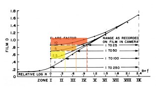
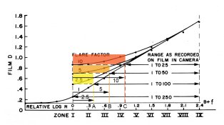
I've been trying to create an example to illustrate why combining flare and the film curve can be misleading. Flare increases the exposure coming from the subject. The x-axis is concerned with log exposure (log-H). Increasing exposure moves the placement to the right. Flare simply moves the shadow exposure to the right where it falls slightly higher on the curve.

What a flare-film curve combination does is project the density from the point where the flare exposure falls to the non-flare subject position. In the example, the exposure from flare is shown using the three colored vertical lines. Everything to the left of those lines actually received no exposure.

 

[Bill Burk]

Everything to the left of those lines actually received no exposure.

I thought everything to the left of those lines simply could not be measured because lesser exposures were wiped out by flare.

 

[Stephen Benskin]

I thought everything to the left of those lines simply could not be measured because lesser exposures were wiped out by flare.

That's the part which is the construct. It doesn't really exist. What actually happens is flare adds to the shadow exposure. This moves it to the left. In the example for a 2.5 flare factor, the shadow exposure shifts from relative log-H 0 to point A. A 5 filter factor shifts the shadow exposure to B and a filter factor of 10 shifts it to point C. The shadow exposure no longer reaches down to relative log-H 0.

 

[markbarendt]

Stephen I think that having the dual legend with density and zone both defining the x axis is a problem.